Lesson 8: Schrödinger equation

How to arrive at the Schrödinger equation

8.1 Mathematical description of quantum objects – 8.2 Preparation of electrons for a specific momentum and kinetic energy
8.3 The wave function of a free electron – 8.4 Operators for physical quantities – 8.5 The kinetic energy operator – 8.6 The eigenvalue equation
8.7 The total energy operator – 8.8 The fundamental equation of quantum mechanics – 8.9 Finding stationary states with the Schrödinger equation
8.10 Progress check – 8.11 Summary

In this chapter, we move from the qualitative to the quantitative consideration of quantum objects. We expand the description of quantum objects by wave functions and introduce operators and eigenvalue equations. We thus come to the eigenvalue equation of the total energy, the Schrödinger equation.
If you have not already done so, please now download Chapter 8 of the teaching materials as a pdf file.

8.1 Mathematical description of quantum objects

The general objectives of physics can be roughly subdivided into two categories:

Qualitative understanding, i. e. to gain an insight into the fundamental cause-effect relationships of natural phenomena. Example: The same fundamental force is responsible for the motion of the Moon around the Earth and the dropping of a stone which has been let go.
Quantitative understanding, i. e. quantitative description of natural phenomena.
Example: Deriving the trajectory of a stone which has been thrown or the motion of the Moon from Newton’s laws.

The preceding chapters concentrated on the qualitative understanding of quantum mechanics. They introduced the concepts of

the wave function $\psi(x,t)$ and
the probability density function $P(x,t) = \left| \psi(x,t) \right|^2$ .

In this chapter, we are looking for the explicit mathematical form of the wave function for a given ensemble of quantum objects. This will lead us to the Schrödinger equation.

8.2 Preparation of electrons for a specific momentum and kinetic energy

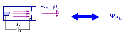
As a preliminary consideration, we consider the preparation of an ensemble of electrons for a specific momentum or kinetic energy.

Electrons can be prepared for a specific momentum or kinetic energy in a cathode beam tube when they pass through an accelerating voltage.

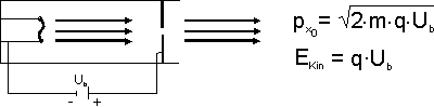
Preparation of the property kinetic energy

8.3 The wave function of a free electron

What does the wave function for an ensemble of electrons with a specific momentum look like?

The simplest approach is a harmonic wave, which is known from classical wave mechanics:

$\psi_{px}(x,t) = A \cdot sin \left( \frac{2 \pi x}{\lambda} - \frac{2 \pi t}{T} \right) + B \cdot cos\left( \frac{2 \pi x}{\lambda} - \frac{2 \pi t}{T} \right)$

$A$ and $B$ are constant factors. The term $(2 \pi \cdot t/T)$ in the argument of the sine or cosine term represents the time dependence of the wave.

In Section 5.3 a wavelength, the de Broglie wavelength, was assigned to the electrons on the basis of the interference phenomena:

$\lambda = \frac{h}{p_x} = \frac{h}{ \sqrt{2mE_{kin}}}$

With the de Broglie wavelength and the abbreviation

$\hbar = \frac{h}{2 \pi}$

we get:

The wave function which is assigned to an ensemble of quantum objects prepared for a specific momentum $p_{x_0}$ is:

$\psi_{pA}(x,t) = A \cdot sin \left( \frac{p_x}{\hbar} \cdot x - \frac{2 \pi t}{T} \right) + B \cdot cos \left( \frac{p_x}{\hbar} \cdot x - \frac{2 \pi t}{T} \right)$

Accordingly, the result for a specific energy Ekin is:

$\psi_{E_{kin}}(x,t) = A \cdot sin \left( \frac{\sqrt{2mE_{kin}}}{\hbar} \cdot x - \frac{2\pi t}{T} \right) + B \cdot cos \left( \frac{\sqrt{2mE_{kin}}}{\hbar} \cdot x - \frac{2\pi t}{T} \right)$

Complex numbers can be avoided in class.

8.4 Operators for physical quantities

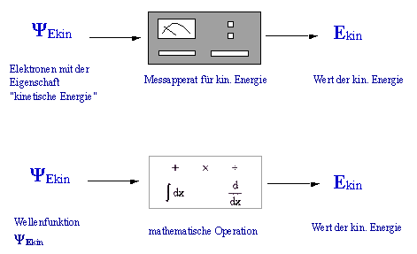
We know that, in an experiment, the quantum objects must first be brought into the desired state by preparation. This experimental “production” of a specific state by means of preparation corresponds on the theoretical side to providing the wave function.

If you have an ensemble which has been prepared for kinetic energy, you want to ascertain the value of the kinetic energy. In an experiment, this is done by means of a measurement. In the theory, this is done mathematically by means of an operator.

Operators:

An operator is the instruction to carry out a certain mathematical operation on the wave function $\psi(x)$ . The application of an operator $\hat{A}$ to the wave function $\psi(x)$ is symbolized by $\hat{A} \cdot \psi(x)$ .

Examples:

Multiplication of a constant:
If the operator $\hat{A}$ means “multiply by a constant $c$ ”, then $\hat{A} \cdot \psi(x)$ stands for $c \cdot \psi(x)$ .
Differentiation of the wave function:
If the operator $\hat{C}$ means “differentiate according to $x$ ”, then $\hat{C} \psi(x)$ stands for

$\psi'(x) = \frac{d \psi(x)}{dx}$

.
The illustration below shows the analogy between the measurement and the application of an operator.
Analogy between measurement and application of an operator.

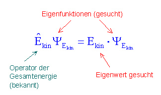
8.5 The kinetic energy operator

How can we obtain the value of the kinetic energy from the wave function for an ensemble of electrons prepared for kinetic energy?

Solving the equation

$\psi_{E_{kin}}(x,t) = A \cdot sin \left( \frac{\sqrt{2mE_{kin}}}{\hbar} \cdot x - \frac{2\pi t}{T} \right) + B \cdot cos \left( \frac{\sqrt{2mE_{kin}}}{\hbar} \cdot x - \frac{2\pi t}{T} \right)$

for $E_{kin}$ does not work. We therefore have to find a different solution.

We place two demands on the kinetic energy operator:

$\hat{E}_{kin} \psi_{E_{kin}} \begin{matrix} \\ \nearrow \\ \searrow \\ \\ \end{matrix} {\displaystyle {\begin{aligned} &\left \text{reproduces} \: \psi_{E_{kin}}\\ \\ &\left \text{returns value from} \: E_{kin} \end{aligned}$

Applying the operator to the wave function should reproduce it apart from a constant factor.
When the operator is applied, it should provide the information on the value of the kinetic energy.

The operation “differentiate twice” fulfils the desired conditions:

$- \frac{\hbar^2}{2m} \frac{d^2}{dx^2} \psi_{E_{kin}}(x) = E_{kin} \cdot \psi_{E_{kin}}(x)$

The kinetic energy operator is

$\hat{E}_{kin} = - \frac{\hbar^2}{2m} \frac{d^2}{dx^2}$

.
If it is applied to a wave function which describes an ensemble of quantum objects with a specific kinetic energy, the wave function is reproduced; the proportionality factor represents the value of the kinetic energy:

$\hat{E}_{kin} \cdot \psi_{kin}(x) = E_{kin} \cdot \psi_{kin}(x)$

.
Note: On the left-hand side of the equation is an operator, but on the right-hand side there is a number.

8.6 Eigenvalue equation

With the operator concept for a physical quantity, we can now answer a question we had considered earlier from a mathematical point of view: Does an ensemble of quantum objects have the property considered?

With the operator $\hat{E}_{kin}$ we can answer the following question:
Do the quantum objects which are described by a specific wave function $\psi(x)$ have the property “kinetic energy” or not?

When the wave function fulfills the eigenvalue equation

$\hat{E}_{kin} \cdot \psi_{kin}(x) = E_{kin} \cdot \psi_{kin}(x)$

,
the quantum objects really do have the property “well-defined kinetic energy”. The value of the kinetic energy which can be ascribed to the quantum objects in this case is given by the proportionality factor $E_ {kin}$ (eigenvalue of the kinetic energy).
If the eigenvalue equation is not fulfilled, the quantum objects described by ψ(x) do not have the property “well-defined kinetic energy”.

Example (Gaussian wave function): $\psi_{Gau\ss} \sim e^{- \frac{(x-x_0)^2}{2 \sigma^2}}$ is a wave function which describes an ensemble of quantum objects which does not have the property kinetic energy. If we apply the kinetic energy operator, the result cannot be written in the form

$\hat{E}_{kin} \cdot \psi_{Gau\ss}(x) = \text{constant} \: \cdot \psi_{Gau\ss}(x)$

The eigenvalue equation is therefore not fulfilled.

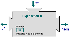
Eigenvalue equation as a machine

Notes:

We can consider the eigenvalue equation to be a “machine”: If we feed a wave function into the machine, it displays whether quantum objects in the state $\psi$ possess the property $A$ or not.
When the eigenvalue equation is fulfilled, the value $E_{kin}$ is definitely found in a measurement. This is exactly the meaning of the expression “possesses the property kinetic energy”.
When the eigenvalue equation is not fulfilled, the measured values have a spread when the kinetic energy is measured.

8.7 The total energy operator

In classical physics, the total energy is the sum of kinetic energy and potential energy. What is the situation in quantum mechanics, where physical quantities are described by operators?

To answer this question, we consider the following thought experiment (it is an expansion of the experiment with the cathode ray tube, Lesson 8.2):
The electrons have been prepared for a fixed energy by the accelerating voltage (region $I$ ). If the electron beam now passes through a further accelerating voltage U, the electrons have a different energy $E_{kin}^{(III)}$ in region $III$ .

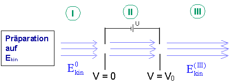
Electrons prepared for kinetic energy again pass through an accelerating voltage

	Description of the potential Potential profile	Potentialverlauf
Region I	The potential has the constant value zero.	$V(x) = 0$
Region II	The electrons are accelerated.	$V(x) \sim x$
Region III	The potential has the constant value $V_0$ . The emerging electrons possess the property “kinetic energy”.	$V(x) = V_0 \: \text{with} \: V_0 \le 0$ .

The graph shows the profile of the potential:

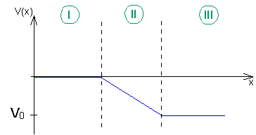
Potential profile in regions I – III.

The detailed consideration about the form of the total energy operator can be found in the teaching materials. Here a brief summary:

First we look for the wave function in a constant potential $V_0$ . It is

$\displaystyle {\psi_{E_{kin}}(x,t) = A \cdot sin \left( \frac{\sqrt{2m(E_{ges}-V_0)}}{\hbar} \cdot x - \frac{2\pi t}{T} \right) + B \cdot cos \left(\frac{\sqrt{2m(E_{ges}-V_0)}}{\hbar} \cdot x - \frac{2\pi t}{T} \right)}$

We again demand that applying the total energy operator should reproduce the wave function.

The total energy operator is

$\hat{E}_{ges} = - \frac{\hbar^2}{2m} \frac{d^2}{dx^2} + V(x)$

.
It is made up of the kinetic energy operator together with the potential energy operator:

$\hat{E}_{ges} = \hat{E}_{kin} + \hat{E}_{pot}$

The operator $\hat{E}_{pot}$ here simply means multiplying the wave function by $V(x)$ .

8.8 The fundamental equation of quantum mechanics

We have now arrived at a crucial point of quantum mechanics. With the concept of the eigenvalue equation and the total energy operator, we can now draw up the fundamental equation of quantum mechanics, the Schrödinger equation.

First a new term here: States in which the probability density function $|\psi(x)|^2$ does not change over time are called stationary states. They are so important because they do not exchange any energy with the environment. They have the property “total energy”.

To find stationary states, we have to solve the eigenvalue equation of the total energy

$\left[ - \frac{\hbar^2}{2m} \frac{d^2}{dx^2}+V(x) \right] \psi(x) = E_{ges} \cdot \psi(x)$

.
It is called the stationary Schrödinger equation and is one of the most important equations of quantum mechanics.

A state with the time-independent probability density $|\psi(x)|^2<span style="font-size: 13.3333px;">$ is called a stationary state. Quantum objects in stationary states possess the property “total energy”. Their wave function $\psi(x)$ fulfills the Schrödinger equation, i. e. the eigenvalue equation for the total energy

$\left[ - \frac{\hbar^2}{2m} \frac{d^2}{dx^2}+V(x) \right] \psi(x) = E_{ges} \cdot \psi(x)$

8.9 Finding stationary states with the Schrödinger equation

So far, we have used the eigenvalue equation to check whether an ensemble of quantum objects described by the wave function $\psi(x)$ possesses a property.
We now want to find the wave function which assigns the property “total energy” to ensembles by solving the Schrödinger equation.

Procedure:

1. Analyze the physical situation:

Find the equation of the potential $V(x)$ .

2. Insert the potential into the Schrödinger equation:

We thus obtain an equation which $\psi(x)$ has to fulfill if it is to have the property “total energy”.

3. Solve the Schrödinger equation:

The wave function $\psi(x)$ can be found by solving the eigenvalue equation. Solving this differential equation is often complicated. One therefore turns to simple models or to approximation methods.

Approach for solving the Schrödinger equation

Here you can find a collection of tasks for quantum mechanics.

8.10 Progress check

The following points were important in this chapter:

What is an operator?
What is the kinetic energy operator and how is it derived?
What is understood by an eigenvalue equation and an eigenvalue?
What form does the total energy operator have?
What form does the Schrödinger equation take and what does it say?
What is the procedure for finding stationary states?

Before you move on to the next chapter, make sure you know the fundamental ideas behind these points. You can then check this with the aid of the Summary.

8.11 Summary of Lesson 8: How to arrive at the Schrödinger equation

In the course so far, the description of electrons with wave functions was purely qualitative. In Chapter 8 we move to the quantitative description, i. e. we are looking for the explicit mathematical form of the wave functions.

The wave function of an ensemble prepared for kinetic energy is:

$\displaystyle {\psi_{E_{kin}}(x,t) = A \cdot sin \left( \frac{\sqrt{2mE_{kin}}}{\hbar} \cdot x - \frac{2\pi t}{T} \right) + B \cdot cos \left(\frac{\sqrt{2mE_{kin}}}{\hbar} \cdot x - \frac{2\pi t}{T} \right)}$ .

The eigenvalue equation for this property tests whether a wave function describes quantum objects with a certain property (e. g. kinetic energy). The eigenvalue equation for the kinetic energy is:

$\hat{E}_{kin} \cdot \psi_{kin}(x) = E_{kin} \cdot \psi_{kin}(x).$

Here $\hat{E}_{kin}$ is the kinetic energy operator:

$\hat{E}_{ges} = - \frac{\hbar^2}{2m} \frac{d^2}{dx^2}$

The stationary Schrödinger equation

$\left[ - \frac{\hbar^2}{2m} \frac{d^2}{dx^2}+V(x) \right] \psi(x) = E_{ges} \cdot \psi(x) .$

is the eigenvalue equation of the total energy. Its solutions are the stationary states, whose probability of finding a particle is constant in time.