9.1 States – 9.2 Operators – 9.3 Expectation values – 9.4 Commutation relations – 9.5 Progress check – 9.6 Summary
This lesson is intended to serve as a brief “refresher” for the quantum mechanical formalism. The theoretical elements which will be introduced in the subsequent chapters are to be put into a more general context. The most important elements of the quantum mechanical formalism are therefore summarized in a brief overview.
9.1 States
In classical mechanics, the state of a body is specified by giving its position and velocity at a specific point in time t. Newton’s laws can be used to derive the further motion of the body from this information. Its trajectory can be calculated from the initial conditions established by the initial preparation.
In quantum mechanics, the key object is the wave function  , which was already introduced qualitatively in Lesson 5. If the mathematical form of the wave function is known, the information on the system concerned is complete. We can calculate probability distributions, expectation values and spreads for each observable.
How can we actually tell from quantum objects which wave function describes them? The wave function is not a quantity which can be measured directly. This is already evident from the fact that it generally has complex values. This means no measuring instrument can exist from which we can read off the value of “ ” directly.
Here the concept of preparation shows yet again how useful it is, because the preparation procedure to which an ensemble of quantum objects is subjected determines its state, i. e. its wave function.
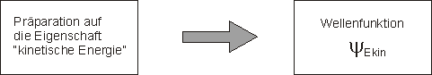
As an example, we come back to the electrons which have been prepared for the property “kinetic energy” in the electron beam tube (Lesson 8). They are assigned the wave function  , i. e. the eigenstate of the kinetic energy, which has the prepared value of the kinetic energy as its eigenvalue.
The preparation determines the wave function of an ensemble of quantum objects.
Preparation here does not always have to mean an artificial process created in the laboratory: Quantum objects can also be prepared “spontaneously”. Excited states of atoms are not long-lived, for example. We can therefore assume that atoms are in the ground state when we can exclude that excitations by collisions, light or similar are taking place. The ground state of atoms is thus prepared spontaneously.
As a solution of the Schrödinger equation, a state  is thus defined apart from a multiplicative constant. The state
  with the (complex) constant is also a solution of the Schrödinger equation.
Usually, the constant is not left undetermined, however, and instead the wave function is normalized. The requirement imposed is:
![\[ \int_V dV \psi^*(\vec{x}) \cdot \psi(\vec{x})=1 \]](https://www.milq.info/wp-content/ql-cache/quicklatex.com-b3c364ae00a444a0f49f91c2c7a49c4a_l3.png "Rendered by QuickLaTeX.com")
The interpretation of this equation is obvious:  is the probability density of finding the electron in the volume element
  around the position vector
  in a measurement. The normalization of the wave function is specified such that the probability that an electron will be found somewhere within the volume under consideration in a measurement becomes one.
9.2 Operators
In quantum mechanics, measured quantities (observables) are described by operators. Some examples of operators (kinetic energy, total energy) have already been discussed in Lesson 8.
The mathematical form of the most common operators can easily be determined with the aid of the following rules:
- We express the corresponding classical quantity by means of position and momentum (e. g.
 )).
)). - We replace
 .
. - Functions of remain unchanged.
The operator for the kinetic energy then becomes:
![\[ \hat{E}_{kin} = - \frac{\hbar^2}{2m} \frac{\partial^2}{\partial x^2} \]](https://www.milq.info/wp-content/ql-cache/quicklatex.com-54ad3df7b275ebbeb2c56110d5c768fb_l3.png "Rendered by QuickLaTeX.com")
in agreement with the result from Chapter 8.
Further examples for operators which can be obtained in this way are:
| Total energy: |
|
| Angular momentum component: |
|
![\[ E_{ges}= \frac{p^2}{2m}+V(x) \rightarrow \]](https://www.milq.info/wp-content/ql-cache/quicklatex.com-527f5929683e1916751a07c8b33b420c_l3.png "Rendered by QuickLaTeX.com")
![\[ \hat{E}_{ges} = - \frac{\hbar^2}{2m} \frac{\partial^2}{\partial x^2} +V(x) \]](https://www.milq.info/wp-content/ql-cache/quicklatex.com-b6c850f33ed036694a13b49a33a921dc_l3.png "Rendered by QuickLaTeX.com")
![\[ L_z = x \cdot p_y - y \cdot p_x \rightarrow \]](https://www.milq.info/wp-content/ql-cache/quicklatex.com-7998139d88b703351aff7d7ff3b47791_l3.png "Rendered by QuickLaTeX.com")
![\[ \hat{L}_z = \frac{\hbar}{i} \left( x \cdot \frac{ \partial}{\partial y} - y \cdot \frac{\partial}{\partial x} \right) \]](https://www.milq.info/wp-content/ql-cache/quicklatex.com-c16a4260dc6e833deb5fcb82a7fedbc1_l3.png "Rendered by QuickLaTeX.com")
In addition, there are also operators (such as the spin operator) whose form cannot be guessed in this way. Here we have to rely on trial and error.
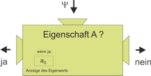
In quantum mechanics, the role of the operators is to extract the information contained in the wave function. One possibility to extract information from the wave function by means of operators has already been discussed: The route via the eigenvalue equation (Lesson 8.6). The eigenvalue equation for operators can furthermore be used to theoretically determine the possible measured values.
We cannot see directly whether the mathematical expression of a wave function describes electrons with the property “kinetic energy” or “angular momentum”. If we want to know, for example, whether an ensemble of electrons which is described by the wave function  possesses the property “kinetic energy”, we apply the kinetic energy operator to the wave function. If it is reproduced, then the eigenvalue equation
  is fulfilled. The electrons concerned then possess the property “kinetic energy”. We can assign a specific value of the kinetic energy (given by the eigenvalue) to each member of an ensemble.
In Lesson 8, the eigenvalue equation was symbolized by a machine with which we can decide whether an ensemble of quantum objects has the relevant property and when this is the case, we can read off its value.
The search for eigenvalues and eigenstates is one of the main tasks in a quantum mechanical problem. The stationary Schrödinger equation is the eigenvalue equation of the total energy, and the reason why we solve it is that we want to theoretically predict the eigenvalues of the energy.
Eigenvalues are therefore important because they are the possible measured values. This has already been discussed in connection with the measurement postulate in Lesson 6. A very specific value is found in each measurement of a physical quantity, i. e. one of the eigenvalues of the quantity measured.
Examples:
- In the double-slit experiment with lamp in Chapter 6, the measured quantity was the position, and each electron was found at a very specific position behind one of the two slits.
- Solving the Schrödinger equation for the hydrogen atom provides only very specific energy eigenvalues. The prediction of quantum mechanics is that only one of these values can be found when the energy is measured.
If we measure the spectrum of a hydrogen atom, we carry out an energy measurement (because  ). The prediction of quantum mechanics is confirmed; only very specific energy values are found.
9.3 Expectation values
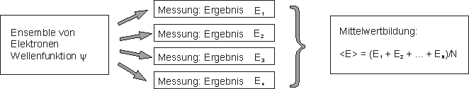
Another type of prediction becomes possible with operators. We can use them to calculate expectation values. In experiments, the expectation value corresponds to the statistical average of a large number of measured values.
In quantum mechanics, the general formula for the expectation value of a physical quantity is
![\[ \langle A \rangle = \int dx \psi^*(x) \hat{A} \psi(x). \hspace{35pt} (1) \]](https://www.milq.info/wp-content/ql-cache/quicklatex.com-038b53e61a3742711e40f46365bc8933_l3.png "Rendered by QuickLaTeX.com")
 here is the operator associated with the physical quantity concerned.
Let us consider an ensemble of quantum objects, e. g. electrons in an electron beam. The electrons are described by the wave function . If we want to calculate the expectation value of the kinetic energy, we need to insert the kinetic energy operator
![\[ \hat{E}_{kin} = - \frac{\hbar^2}{2m} \frac{\partial^2}{\partial x^2} \]](https://www.milq.info/wp-content/ql-cache/quicklatex.com-63f72b94a27c4c4aa36e32efb6346e87_l3.png "Rendered by QuickLaTeX.com")
into Equation (1) and carry out the integration.
What is the meaning of the value we computed using Equation  ? How can it be related to experimental data? This is where the statistical interpretation becomes important again. The expectation value is a statistical quantity which relates to a large number of measurements on different members of an ensemble.
For the example of the kinetic energy, this means in more detail:
1. We require: An ensemble of identically prepared electrons which are described by the wave function
2. We carry out the kinetic energy measurements on a large number of electrons in this ensemble.
3. We calculate the average value of the kinetic energies measured. It must have the same value as the expectation value calculated with Equation within the measuring accuracy.
9.4 Commutation relations
Some operators do not commute. This means: The order in which they are applied to a wave function matters. The best known examples are position and momentum. The following applies for them:
![\[ \hat{p} \hat{x} \psi(x) \neq \hat{x} \hat{p} \psi (x). \]](https://www.milq.info/wp-content/ql-cache/quicklatex.com-3438d606eb2c1bde92d60bcf7f953009_l3.png "Rendered by QuickLaTeX.com")
When we insert the explicit form of the operators, the chain rule gives us:
![\[ {\displaystyle {\begin{aligned} \hat{p} \hat{x} \psi(x) &\left = - i \hbar \frac{d}{dx} \left( x \psi(x) \right) \\ &\left = i \hbar \psi(x) - i \hbar x \frac{d}{dx} \psi(x) \\ &= i \hbar \psi(x) + \hat{x} \hat{p} \psi(x). \end{aligned} \]](https://www.milq.info/wp-content/ql-cache/quicklatex.com-33f016f383c16e37933d8f1ffb75443c_l3.png "Rendered by QuickLaTeX.com")
We can therefore write: ![[ \hat{x}, \hat{p}] \psi(x) \equiv (\hat{x} \hat{p} -\hat{p} \hat{x}) \psi(x) = i \hbar \psi(x)](https://www.milq.info/wp-content/ql-cache/quicklatex.com-234173a595cb7a087580b870a2022d81_l3.png "Rendered by QuickLaTeX.com")
or ![[ \hat{x}, \hat{p}] = i \hbar](https://www.milq.info/wp-content/ql-cache/quicklatex.com-5b9c6ed445f13baaa7c39612493999c2_l3.png "Rendered by QuickLaTeX.com")
The quantity ![[\hat{A}, \hat{B}]](https://www.milq.info/wp-content/ql-cache/quicklatex.com-f88795490b5b591eeacce66352962e99_l3.png "Rendered by QuickLaTeX.com") is called the commutator of the two operators and
is called the commutator of the two operators and  .
.
The mathematical fact that two operators do not commute (their commutator is not zero) would not be worthy of further note were it not for the fact that the uncertainty relation is linked to it.
An uncertainty relation with all the consequences already discussed in Lesson 7 applies to two operators which do not commute. An ensemble of quantum objects cannot be prepared for the two corresponding properties simultaneously, for example.
For two physical quantities  and
and  (e. g. position and momentum) with the commutation relation
 ![[\hat{A}, \hat{B}] = i \hat{C}](https://www.milq.info/wp-content/ql-cache/quicklatex.com-03395d0c3ea268bbdcf838375524fafd_l3.png "Rendered by QuickLaTeX.com")
the uncertainty relation is:
![\[ \Delta A \cdot \Delta B \geqslant \frac{1}{2} \left| \langle \hat{C} \rangle \right| \hspace{35pt} (2) \]](https://www.milq.info/wp-content/ql-cache/quicklatex.com-a936892854e6665f052620e8b5308583_l3.png "Rendered by QuickLaTeX.com")
where and
and  are defined as spreads, as in Chapter 7.
When the two operators commute, the right-hand side becomes zero. Equation  is then reduced to the trivial statement that a product of two positive quantities cannot be negative.
For position and momentum
,
so that the relation
 results again.
9.5 Progress check
When you have worked through this chapter, you should be able to answer the following questions:
- Why is the wave function normalized to one?
- What is the relationship between measured quantities and operators?
- Which rules can be used to obtain quantum mechanical operators from the corresponding classical quantities?
- If, for a physical system, the eigenvalue equation is fulfilled for a specific operator: What does this say about the system concerned?
- How can the possible measured values of an observable be determined theoretically?
- How are expectation values calculated?
What corresponds to the quantum mechanical expectation value in an experiment? - What do we mean by commutation relations?
- What is the physical consequence when two operators do not commute?
9.6 Summary of lesson 9: Overview of the quantum mechanical formalism
The summary here gives you the answers to the questions from the progress check.
- Why is the wave function normalized to one?
 is the probability density of the electrons. The wave function is normalized to one so that the probability of finding an electron somewhere within the volume under consideration in a measurement becomes one:
![\[ \int_V dV \psi^*(\vec{x}) \cdot \psi(\vec{x}) = 1 \]](https://www.milq.info/wp-content/ql-cache/quicklatex.com-ecdb60bcecfdcde7c9d7b5ef5833faeb_l3.png "Rendered by QuickLaTeX.com")
- What is the relationship between measured quantities and operators?
In quantum mechanics, an operator is assigned to each measured quantity. With the rules introduced in this chapter, theoretical predictions can be made about the measured quantity concerned (e. g. expectation values or the possible measured values can be calculated). - Which rules can be used to obtain quantum mechanical operators from the corresponding classical quantities?
We replace by in the classical expression; functions of x remain unchanged. - If, for a physical system, the eigenvalue equation is fulfilled for a specific operator: What does this say about the system concerned?When the eigenvalue equation for the kinetic energy is fulfilled, for example, this means that the electrons concerned actually have the property “kinetic energy”. A very specific value is found in each measurement of the kinetic energy.
- How can the possible measured values of an observable be determined theoretically?
The possible measured values of an observable are its eigenvalues. So these need to be computed. For electrons in the Coulomb potential (H atom), for example, there are very specific eigenvalues of the total energy. Only these values are found in energy measurements, which becomes apparent in the appearance of line spectra, for example. - How are expectation values calculated?
The equation is .
. - What corresponds to the quantum mechanical expectation value in an experiment?
- In an experiment, the expectation value corresponds to the statistical average of a very large number of measured values of the quantity observed which were obtained using identically prepared quantum objects.
- What do we mean by commutation relations?
For a lot of operators, the order in which they are applied to a wave function matters. The commutation relations express this formally. - What is the physical consequence when two operators do not commute?
For two operators which do not commute, the uncertainty relation
 , applies, where
 ![\left[ \hat{A}, \hat{B} \right] = i \hat{C}](https://www.milq.info/wp-content/ql-cache/quicklatex.com-e2e1289c98da0209d418f0c2771f584d_l3.png "Rendered by QuickLaTeX.com") .
.