Lesson 5: Electrons as quantum objects

5.1 Electron diffraction – 5.2 Double-slit experiment with electrons and atoms – 5.3 Wavelength of electrons
5.4 Double-slit experiment with classical particles and electrons – 5.5 Probabilistic interpretation and wave function
5.6 Wave function and probability distribution for the double-slit experiment- 5.7 Progress check – 5.8 Summary

The considerations undertaken in the previous lessons using the example of photons are now repeated in a similar way using the behavior of electrons as the quantum objects, but this time in more depth and in more detail. The wave function and the probability density function are introduced and the naive wave-particle duality is replaced by the Born probabilistic interpretation.

The experiments considered in this lesson can again be carried out with the “double-slit” simulation program. If you have not yet downloaded the “Doppelspalt.exe” simulation program (in Lesson 4.0), choose the menu entry The materials – downloads – simulations programs – 4th simulation program for the double-slit experiment

If you have not already done so, please now download Chapter 5 of the teaching materials as a pdf file.

5.1 Electron diffraction

The experiment with the electron diffraction tube demonstrates that electrons also exhibit wave behavior.

Experiment 5.1: In an electron tube (Fig. 5.1 a) the cathode, which is heated with $6 V$ , emits electrons. These electrons pass through an accelerating voltage $U_B = 5 kV$ . They are collimated by the electrodes K1, K2 and A1, which are arranged one behind the other, to form an electron beam. Anode A2 has a bored hole holding a thin film of polycrystalline graphite through which the beam passes. On the fluorescent screen, several bright rings can be seen around a central spot in the middle (Fig. 5.1 b). Increasing $U_B$ brings about a decrease in the radii.

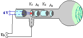
Fig. 5.1.1 a) Electron diffraction tube

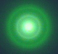
Fig. 5.1.1 b) Electron diffraction pattern on the screen

The bright rings are caused by electron diffraction. As is the case with the Bragg diffraction of X-rays, the electrons are diffracted by the crystal lattice of the graphite. This diffraction phenomenon is a strong indication that the electrons exhibit wave behavior in addition to their well-known particle behavior.

The result of the experiment can be summarized as follows:

The bright rings are caused by electron diffraction. This is a strong indication that the electrons exhibit wave behavior in addition to particle behavior.

5.2 Double-slit experiments with electrons and atoms

We observe interference phenomena at the double slit with electrons as well: Start the simulation program for the double-slit experiment and carry out Experiments 5.2 and 5.3 described in the teaching materials.

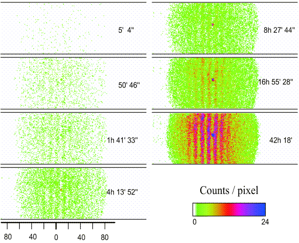
In Experiment 5.2 you conduct the double-slit experiment with electrons (using the same specifications as in the real experiment by Claus Jönsson, Univ. of Tübingen 1961), in Experiment 5.3 with helium atoms, which are more than ten thousand times bigger. In the top figure, the emergence of an interference pattern from individually detected helium atoms can be observed with the aid of original experimental data (Univ. of Constance 1991). In the case of the experiment with electrons, the result looks similar. In both experiments, the behavior of the particles is completely analogous to that of the photons (cf. Lesson 4.2): The individually detected particles transfer all their energy to a single point on the screen and leave behind individual, point-like spots at apparently random positions, which emphasizes the particle character. The more particles are detected, the clearer the distribution evolves into the characteristic wave phenomenon of the well-known double-slit interference pattern. But if it really were a pure wave phenomenon, the interference pattern would have to appear as a whole on the screen right from the start, albeit very weakly.

The results of the experiments lead to the following conclusion:

If the electrons exhibited pure wave behavior, the interference pattern would appear on the screen immediately as a whole, albeit with a very weak intensity. Instead, a well-defined amount of energy is released each time at a specific position on the screen, as is characteristic for particle-like behavior.

Neither a pure wave model nor a pure particle model describes the behavior of the electrons.

The development of the matter wave interferometer

Here you can download a worksheet on the behavior of electrons or atoms at the double slit.

5.3 The wavelength of electrons

If particles, i. e. electrons for example, have wave properties, as explained in Lesson 5.2, then it should be possible to assign a wavelength to these electrons. This was the (not yet experimentally confirmed) initial consideration of Louis-Victor de Broglie (pronounced: ´Broej´) in his 1924 doctoral thesis. He equated the energy-mass equivalence (( $E = m \cdot c^2$ ) with the photon energy ( $E_{Phot} = h \cdot f$ ). Via the momentum $p = m \cdot c$ , which represents a typical particle quantity, and the fundamental equation of wave mechanics $c = \lambda \cdot f$ , we obtain the

de Broglie relationship between wavelength and momentum:

$\displaystyle{p = \frac{h}{\lambda}}$

$\displaystyle{\lambda = \frac{h}{p}}$

The wave behavior of electrons is characterized by the de Broglie wavelength $\lambda$ . Characteristic for this equation is the linking of the classical “particle property” $p$ (momentum) with the classical “wave property” $\lambda$ (wavelength) via Planck’s constant $h$ .

It took a few years before it was possible to check this relationship by means of an experiment with the electron diffraction tube, whose derivation and explanation you will find in Chapter 5 of the lecture notes download (The materials – lecture notes).

In fact, we find electron wavelengths (as a function of the kinetic energy) in the double-digit picometer range ( $\approx 1,7 \cdot 10^{-11}m$ ) via the radii of the diffraction rings in the experiment with the electron diffraction tube (Lesson 5.1) and the lattice plane separations d of the irradiated graphite crystal using the Bragg relationship.

5.4 Double-slit experiment with classical particles and with electrons

Let us again consider the behavior of classical particles at a double-slit: Use the mouse to press on the “nozzle” of the paint spray can. The droplets of the spray can represent the classical particles here.

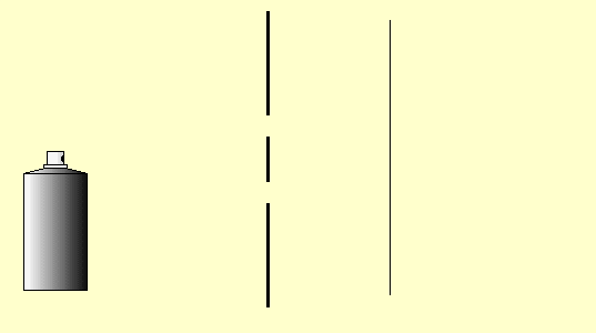
You can carry out this little simulation of classical particle behavior at the double slit with the double-slit simulation program (Experiments 5.4 and 5.5 in the lecture notes) (cf. Simulation program for the double-slit experiment) or as a real experiment as well. Cut two slits in a sheet of paper or cardboard with a sharp blade and spray small paint droplets from a paint spray can through this double slit onto the paper screen behind it.

Observation: The intensity of the paint on the screen is greatest behind the slits (if they are not too far apart, as in the simulation above) and decreases continuously towards the outside and without any obvious structures (Fig. 5.4.1 (a)). We describe the distribution of the paint intensity by means of the function $P(x)$ (Figure (d)), which is produced as the sum of the individual slit distributions (one slit open, the other one closed: Figures (b) and (c)), as can be seen from Figure (5.4.1) below.

The following applies: $P(x) = P_1(x) + P_2(x)$ .

5.4.1 Double-slit experiment with paint droplets (classical particles)

If the same experiment is carried out with electrons (Experiment 5.6 in the lecture notes), a similar distribution pattern results in each case when one slit is opened on its own (cf. Figures 5.4.2 (b) and (c) below). If we open both slits, however, the resulting overall distribution is different to that for classical particles. We can now see an interference pattern instead of a sum distribution.

The following therefore applies to electrons: $P(x) \neq P_1(x) + P_2(x)$ .

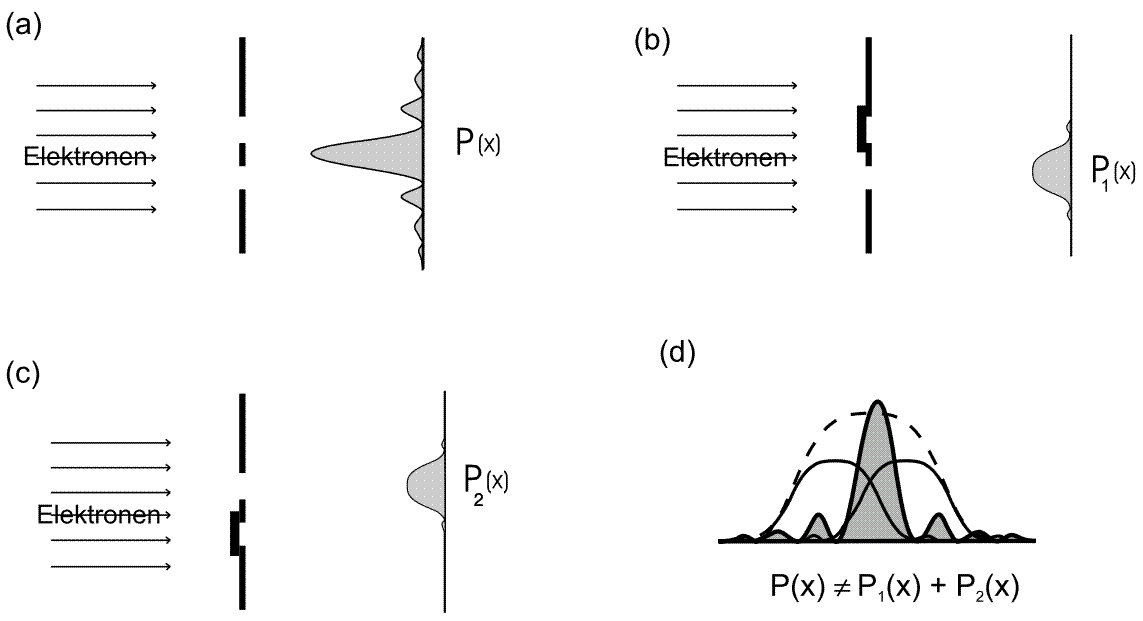
Fig. 5.4.2 Double-slit experiment with electrons

The remarkable feature here is that several intensity minima are formed in this overall distribution which are not present in the individual slit distribution. The electrons therefore have a different distribution depending on whether the other slit is also open or not.

We note the following:

With classical particles, the distribution at the double slit is simply the sum of the individual distributions:

$P(x) = P_1(x) + P_2(x)$ .

This is not the case for quantum objects:

$P(x) \neq P_1(x) + P_2(x)$

This strange behavior will be investigated further now.

Here you can download a worksheet on the intensity distributions at the double slit.

5.5 Probabilistic interpretation and wave function

In the experiments discussed in the last section (5.4), the intensity distribution of the electrons was characterized by a distribution function $P(x)$ which stated how high the intensity was at a specific position $x$ . In quantum mechanics, this distribution function is interpreted as a probability density $P(x)$ . When multiplied by $\Delta x$ (or $\Delta V$ ) it says something about the probability of finding an individual quantum object in the interval $\Delta x$ (or in the spatial region $\Delta V$ ) around the position x in a measurement (e. g. at a certain position on the screen behind a double slit). We can only make statistical statements about individual quantum mechanical events (cf. Lesson 4.2): If the probability density is very high, the probability of finding the object there is very high; if it is zero, we will never find a quantum object there.

With the aid of the probability density function $P(x)$ , we can describe quantum objects such as electrons and photons (in large numbers). For example, we can thus predict the distribution of an identically prepared ensemble (definition cf. Lesson 4.3) of electrons on the screen with the double-slit experiment if the probability density function $P(x)$ is known. A probabilistic statement can thus be verified experimentally as well by detecting the relative incidences with the aid of detectors and representing them graphically by histograms, for example. The objective of mathematical calculations in quantum mechanics is to determine the probability function $P(x)$ in the particular physical situation of interest.

It has turned out to be advantageous to not work with $P(x)$ itself, but with a function $\psi(x)$ , which is called a wave function. We obtain $P(x)$ from $\psi(x)$ by squaring it: $P(x) = |\psi(x)|^2$ .

It is advantageous to work with the wave function $\psi(x)$ instead of $P(x)$ , because:

> The interference phenomenon can be explained with $\psi(x)$ .
> The particle character is covered by the probabilistic interpretation of $P(x) = |\psi(x)|^2$ .
> The wave function is assigned to an ensemble of identically prepared quantum objects.
> $\psi(x)$ can be determined with the aid of the Schrödinger equation.
> The temporal evolution of $\psi(x)$ can be calculated more easily.
> $\psi(x)$ obeys the superposition principle.

The wave function $\psi(x)$ is assigned to an ensemble of identically prepared quantum objects and propagates according to the rules of classical wave mechanics with its typical phenomena such as diffraction or interference. Quantum objects (e. g. electrons and photons) are described by a wave function $\psi(x)$ ; this explains the wave character of quantum objects. In contrast, $|\psi(x)|^2 \cdot \Delta x$ (or for the region of space: $|\psi(x)|^2 \cdot \Delta V$ ) gives the probability of detecting an electron at a specific position, i. e. as a particle (spot registration on a screen).

The probabilistic interpretation, which was formulated by Max Born (1926), and the way it links wave-like propagation and particle-like detection, thus explains the result of the double-slit experiment: The emergence of the interference pattern from individual spots. It is no longer necessary to describe the behavior of quantum objects by means of either a wave model or a particle model. The naive wave-particle duality is thus overcome.

Born probabilistic interpretation:

Quantum objects are described by a wave function $\psi(x)$ . The wave function determines the probability of detecting a quantum object in the interval $\Delta x$ around the $position \: x$ :

$P(x) \cdot \Delta x = |\psi(x)|^2 \cdot \Delta x$ .

With the aid of the Born probabilistic interpretation, the apparently incomprehensible behavior of quantum objects becomes clearer: Although it is impossible to predict the position of an individual quantum object, the probability density $P(x)$ can be predicted. For an ensemble of quantum objects, it corresponds to the distribution of the relative incidences. The wave function $\psi(x)$ combines the wave-like propagation of the wave function and the particle-like behavior as the quantum objects are being detected in a unified concept. This means the naive wave-particle duality is overcome.

Here you can download the article “Die Ensemble-Interpretation der Quantenmechanik (The ensemble interpretation of quantum mechanics)”.

5.6 Wave function and probability distribution in the double-slit experiment

In Experiment 5.6 (cf. Lesson 5.4) we saw that the distribution $P(x)$ does not correspond to the sum of the individual distributions $P_1(x)$ and $P_2(x)$ for the double-slit experiment with electrons.

$P(x) \neq P_1(x) + P_2(x)$

This result can be easily understood with the aid of the wave function: According to classical wave theory, the two waves superimpose, as can be observed happening on the surface of a lake, for example, when two stones are thrown into the water not too far away from each other. Mathematically, this is expressed by adding the two wave functions:

$\psi(x) = \psi_1(x) + \psi_2(x)$ .

We say that the quantum objects described by such a wave function are in a superposition state of $\psi_1(x)$ and $\psi_2(x)$ , which results from the addition of two wave functions.

The probability function $P(x)$ of the superposition state is obtained by squaring the absolute value of the wave function1:

$P(x) = |\psi_1(x) + \psi_2(x)|^2$

$P(x) = |\psi_1(x)|^2 + |\psi_2(x)|^2 + 2 \cdot \psi_1(x) \cdot \psi_2(x)$

The last term in the sum is called the interference term. It is responsible for the fact that we find an electron distribution in the double-slit experiment with two open slits, where the following applies:

$P(x) \neq P_1(x) + P_2(x)$

and which explains why we cannot simply add the two single-slit distributions (cf. Fig. 5.4.2 in Lesson 5.4).

¹ The assumption here is that the wave function has real values. In the case of complex wave functions, the following applies:

$P(x) = |\psi_1(x)|^2 + |\psi_2(x)|^2 + \psi_1(x) \cdot \psi_2^*(x) + \psi_1^*(x) \cdot \psi_2(x)$ .

5.7 Progress check

The following points were important in this chapter:

Wave behavior of electrons: Electron diffraction.
Behavior of electrons and atoms at the double slit.
Wavelength of an electron.
Comparison of the intensity distributions for classical particles and electrons.
Concepts: Probability density function, wave function and Born probabilistic interpretation.
Before you move on to the next chapter, make sure you know the fundamental ideas behind these points. You can then check this with the aid of the Summary.

5.8 Summary of Lesson 5: Electrons as quantum objects

After the photons in the last chapters, this chapter discusses electrons as further quantum objects.

Electrons exhibit interference phenomena in the electron diffraction tube and in the double-slit experiment. This is still the case even when the experiment is carried out with individual electrons.

Electrons with momentum p can be assigned a wavelength $\lambda = h/p$ .

In the double-slit experiment, the distribution of the electrons $P(x)$ is not equal to the sum of the two individual slit distributions (as is the case for classical particles). The following applies:

$P(x) \neq P_1(x) + P_2(x)$ .

A key element for the theoretical description of quantum objects is the wave function $\psi(x)$ .

Born probabilistic interpretation:
Quantum objects are described by a wave function $\psi(x)$ . The wave function determines the probability of detecting a quantum object in the interval $\Delta x$ around the position $x$ :

$P(x) \cdot \Delta x = |\psi(x)|^2 \cdot \Delta x$ .

The Born probabilistic interpretation replaces the naive wave-particle duality.