Lesson 7: Heisenberg’s uncertainty relation

7.1 Simultaneous preparation of different properties – 7.2 Preparation of position and momentum for photons – 7.3 A measure for the “quality” of a preparation
7.4 Measurement method and properties – 7.5 Electrons at the single slit and quantitative expression of the uncertainty relation
7.6 Uncertainty relation and path concept – 7.7 Progress check – 7.8 Summary

The Heisenberg uncertainty relation is often seen as one of the most important insights of quantum mechanics. This chapter shows how it can be expressed as a statement about the ability to simultaneously prepare properties.

You can download the slightly more detailed Chapter 7 of the teaching materials as a pdf file to help you.

7.1 Simultaneous preparation of different properties

In preparation for understanding the Heisenberg uncertainty relation, we will again discuss the preparation of properties concept (preparation).

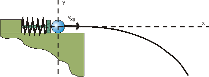
Fig. 7.1.1 Catapult from Chapter 2

Using the example of the horizontal throw, as familiar from the example of the catapult from Chapter 2, we recognize that position and momentum have to be prepared simultaneously to produce identical initial conditions, i. e. identical values of the launch position and the launch velocity.
“Prepare” means that the spread of the measured values is zero or very small when measurements of the prepared quantity are undertaken on an ensemble of balls. This simultaneous preparation for position and momentum, i. e. two properties, does not pose any problems in principle in classical physics.

Although individual properties for an ensemble of quantum objects can be prepared in quantum physics (e. g. polarization properties with photons), it is not possible to prepare several at the same time. Pairs of properties exist (e. g. position and momentum) whose simultaneous preparation is fundamentally impossible, although the preparation of the individual properties does not come up against any fundamental limits. This is the essence of Heisenberg’s uncertainty relation, which is to be explained in more detail in the sections below.

7.2 Preparation of position and momentum for photons

To show the impossibility of the simultaneous preparation of position and momentum, we look at the following experiment where we want to try and produce both properties simultaneously: We use the photons of a monochromatic laser beam as the quantum objects

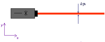
Fig. 7.2.1 Laser beam of a specific width

Since the beam is very well collimated, the momentum component^₁₎ $p_y$ perpendicular to the beam direction (i. e. in the y-direction) for all photons is practically zero; this means that the spread of possible measured values of a large number of photons around the value $p_y= 0$ would be infinitesimal.

The laser beam has a certain spatial width in the y-direction, however. Possible measured values for the position component y therefore have a spread $\Delta y_0$ . The photons are therefore not prepared for the property “position component y”.

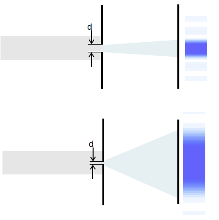
To now carry out this preparation – i.e. to reduce the spread of the position component y – we could make the beam pass through a narrow slit.
We know from wave optics, however: If a laser beam passes through a narrow slit (width d), it becomes wider behind the slit. If the slit width is varied, the following result is achieved: The narrower the slit, the wider the beam becomes.

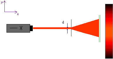
Fig. 7.2.2 Diffraction of a laser beam at a slit aperture

The slit has caused the laser beam to become narrower immediately behind the slit. This means that the measured values of the position component y in the slit plane are not spread as much: The spread has been reduced from $\Delta y_0$ to $\Delta y \approx d$ . This corresponds to an improvement in the position preparation. But unfortunately, the widening of the beam behind the slit shows that the photons are no longer collimated: The photons now have a spread in the transverse direction and have lost their property “momentum component $p_y =0$ ”.

Conclusion: Although it was possible to reduce the position spread of the photons in the y-direction immediately behind the slit with the aid of the slit, the momentum spread has simultaneously been increased in the y-direction. It has been impossible to prepare position and momentum simultaneously.

This is a general principle in quantum mechanics, which can be stated as follows:

Heisenberg’s uncertainty relation:
It is impossible to prepare an ensemble of quantum objects simultaneously in respect of position and momentum.

Discussion regarding the textbook approaches

¹⁾See Chapter 1.4 for photon momentum.

7.3 A measure for the “quality” of a preparation

It is possible to formulate Heisenberg’s uncertainty relation even more quantitatively, i. e. as a relation that states how “well” position and momentum can be prepared simultaneously on an ensemble of quantum objects.
The expression “quality of a preparation” to be clarified can be explained using the example of the single-slit experiment with electrons.

Thought experiment: A beam of electrons is incident on a slit of width d. Immediately behind the slit is a high-resolution detector which can detect the electrons with a resolution which is far higher than the slit width. It registers the number of electrons arriving at a certain point per second (Fig. 7.3.1).

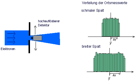
Fig. 7.3.1 Preparation of an electron beam for the property “position”

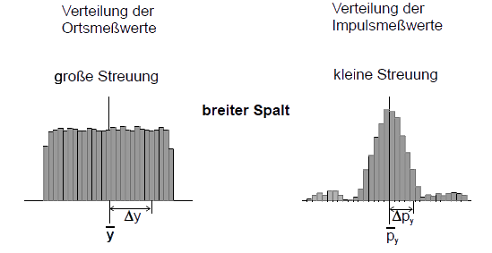
The detector conducts position measurements on the electrons which pass through the slit. To record the distribution of the measured values within this region statistically, we determine their mean value $\overline{y}$ and their standard deviation $\Delta_y$ . The mean value states where the distribution of the measured values has its “geometric center”, the standard deviation is a measure of its spread. The distribution of the measured position values is shown in the figure above. When the slit is relatively narrow, the spread is quite low as well. With a wider slit, the measured position values have a larger spread.

When the spread of the measured values is zero, the preparation is perfect (which can never be achieved in our case, because the slit would then be closed). When the standard deviation is not zero, this means that the measured values have a spread. In this case, the preparation is not perfect and the standard deviation provides information on how much the preparation of the property concerned deviates from an ideal preparation.

The “quality” of the preparation of a property (e. g. position component y) can be assessed with the aid of the spread of the measured values in a test measurement. The smaller the standard deviation Δy of the measured values, the better prepared is the property.

When $\Delta_y =0 \: \Rightarrow$ preparation is perfect (measured values have no spread).

When $\Delta_y \neq 0\: \Rightarrow$ preparation is imperfect (measured values have a spread).

7.4 Measurement method and properties

The relationship between the spread of measured values and the property which an object possesses can be illustrated once again using an analogy from classical physics.
For this purpose we consider round and square metal plates. The round plates have the property “diameter”. Such a property cannot be assigned to the square plates, the question about their diameter is meaningless.

> What happens when we nevertheless try to measure a diameter with the square plates?

Or:

> What is the result when we try to measure a property which the object concerned does not even possess?

To find the answer, we have to invent a measurement method for the property “diameter”. We can measure the distance from edge to edge at different angles with a tape measure. The constraint here is that the tape always has to go through the center of the object.

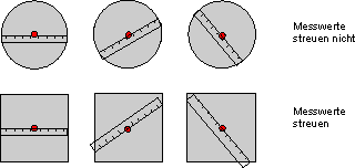
Fig. 7.4.1 Measurement method for the property “diameter”

> We always get the same measured value for the round plates $\Rightarrow$ they possess the property “diameter”.

> For the square plates the measured values have a spread $\Rightarrow$ they do not have this property.

According to the same principle, we can ask for the property “side length”.

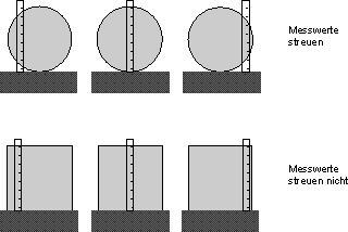
Fig. 7.4.2 Measurement method for the property “side length”

With this measurement method, the measured values for the round plates vary, while we always obtain the same measured value for the square plates, which gives the side length of the plates.

This shows that there are even examples for macroscopic objects where we have to be careful when assigning a property or that there are situations in which the simultaneous preparation of two properties (here: diameter and side length) is impossible.

With quantum objects, we generally have to use a suitable preparation method to ascertain whether the assignment is meaningful for each property.

One example: We can send light through a polarization filter with horizontal orientation (e. g. with the aid of the simulation experiment Polfilter.exe, which you possibly already know from Chapter 2.4). The photons behind the filter are now prepared to have the property “horizontally polarized” (Fig. 7.4.3). A test confirms this (= complete passage through a second, horizontal polarization filter).

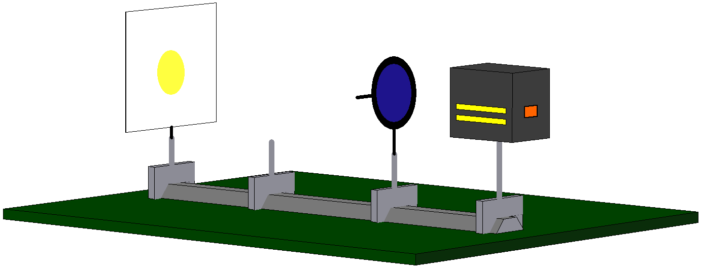
If we now try to additionally prepare these photons for the property “vertically polarized” with the aid of a second polarization filter with vertical orientation (cf. Fig. 7.4.4), we will necessarily fail: Not one single photon passes through the second filter with vertical orientation. There are therefore no photons with the property “horizontally polarized” which are simultaneously prepared for the property “vertically polarized”.

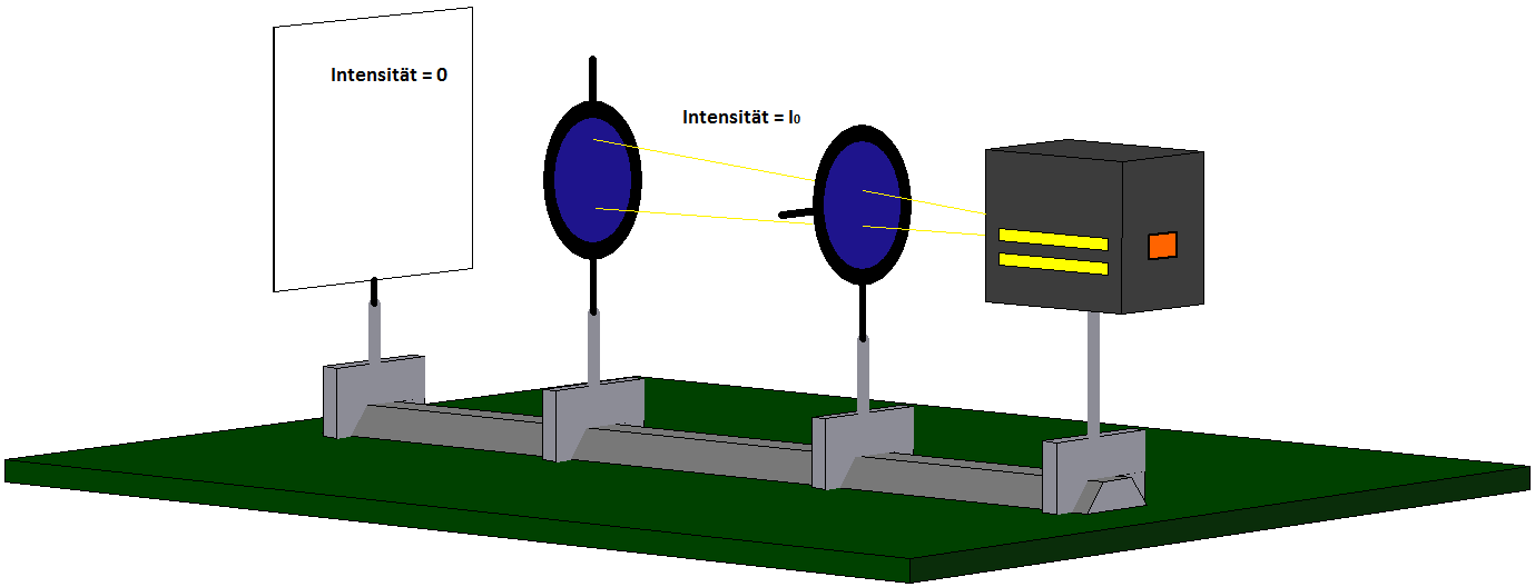
The two properties cannot be prepared simultaneously, they are mutually exclusive properties.

7.5 Electrons at the single slit and quantitative expression of the uncertainty relation

The question is, to what extent are position and momentum preparation mutually exclusive?
Or in other words: Is there a limit to how close we can come to the ideal of a perfect preparation?

Below we want to state Heisenberg’s uncertainty relation quantitatively as a relation between the values for the quality of the preparation of position $(\Delta y)$ and momentum $(\Delta p_y)$ (see Section 7.4 for the corresponding spreads or standard deviations). For this purpose, we again consider the broadened diffraction pattern for an electron beam which passes through a single slit which gets narrower (Fig. 7.5.1, Experiment 7.4 in the lecture notes).

Here as well, the distributions of the measured position and momentum values for an ensemble of electrons are recorded immediately behind the slit (cf. Section 7.3), transferred into a histogram and the standard deviations (position $(\Delta y)$ and momentum spread $(\Delta p_y)$ ) determined. For a wide slit, the result is a relatively large position spread, but a small momentum spread (Fig. 7.5.2).

For a narrow slit, the position spread is now small, but the momentum spread large (Fig. 7.5.3).

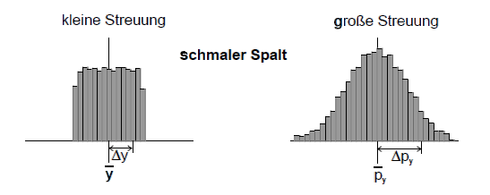
The spread of the measured momentum values increases when the spread of the measured position measurements decreases and vice versa: There seems to be a reciprocal relationship between the two spreads in the example shown. This means: The larger the spread of the transverse momenta (in the y-direction, $p_y$ ), the wider the diffraction image. We can therefore estimate the spread of the measured momentum values at the slit using the width of the diffraction pattern on the screen.

Estimate of the momentum spread

Most electrons are registered on the screen within the principal maximum of the diffraction pattern, i. e. within the angular range between $+ \alpha$ and $- \alpha$ (Fig. 7.5.4). We can therefore limit ourselves to this range to estimate the spread of the transverse momenta $\Delta p_y$ .

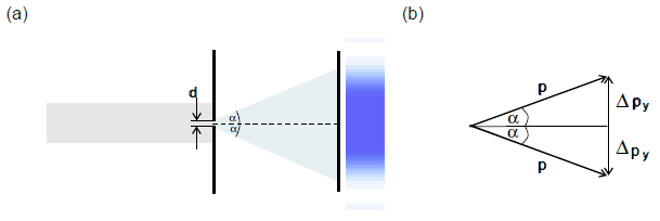
Figure 7.5.4 b) therefore yields:

$\sin \alpha \approx \Delta p_y /p$ or $\Delta p_y \approx p \cdot \sin \alpha$ .

The range of the principal maximum is limited by the first diffraction minima, its position is known from classical optics:

$\sin \alpha = \lambda / d$ .

In the case of electrons, $\lambda$ is the de Broglie wavelength $(\lambda = h/p)$ of the incident beam prepared for the momentum $p$ ; this gives:

$h/ (p \cdot d) \approx \Delta p_y / p$ .

Cancelling $p$ and finally approximating the spread of the measured position values $\Delta y$ by the slit width $d$ ( $d \approx \Delta y$ immediately behind the slit), we then get:

$\Delta y \cdot \Delta p_y \approx h$

In this example, the product of the two spreads is always of the order of Planck’s constant $h \: (h = 6,626 · 10^{-34} Js)$ .

The equation above represents the quantitative expression of the Heisenberg uncertainty relation for the special example of the slit. In its general form, it describes in general how well position and momentum preparation are possible simultaneously:

If we prepare an ensemble of quantum objects in such a way that the spread of the measured position values $\Delta y$ is small, the spread of the measured momentum values $\Delta p_y$ will be large (and vice versa). The following relationship applies:

$\displaystyle{\Delta y \cdot \Delta p_y \ge \frac{h}{4 \pi}}$

Here you will find some additional explanations of the uncertainty relation.

You can download a worksheet here.

The interpretation of the Heisenberg uncertainty relation
(published in “Physik in der Schule” 35 (1997), pp. 176 – 179; pp. 218 – 221).

7.6 Uncertainty relation and trajectory concept

Heisenberg’s uncertainty relation means saying farewell to the concept of the trajectory of a particle as it is used in classical physics.
The trajectory concept is related to the idea that the object simultaneously has a specific position and a specific momentum (velocity) at every point in time, something which is relatively self-evident in classical mechanics.
Quantum objects can never possess the properties “position” and “momentum” at the same time, however. According to Heisenberg’s uncertainty relation, the product of the spreads $\Delta y \cdot \Delta p_y$ must always be of the order of Planck’s constant h or larger.

But how can this be reconciled with the observation that electrons apparently follow a well-defined trajectory in an electron beam tube?

To solve this apparent contradiction, we consider the following example:

In an electron beam tube, the electron beam is reduced to a width of $\Delta y_1 \approx d = o,1 mm$ at the anode (Fig. 7.6.1).

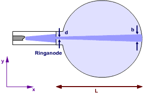
Fig. 7.6.1 “Trajectory” of the electrons in an electron beam tube

The spread of the momenta in the $y$ -direction (i. e. at right angles to the beam direction) is therefore at least:

$\Delta p_y = h / (4 \pi \cdot \Delta y_1) = 5,3 \cdot 10^{-31} kg \: m/s$ .

The velocity spread in the $y$ -direction is obtained by dividing $\Delta p_y$ by the electron mass:

$\Delta v_y = \Delta p_y / m_e = 0,58 m/s$ .

For comparison, we calculate the velocity in the $x$ -direction (i. e. in the beam direction) which an electron possesses for an accelerating voltage of $1 kV$ :

The following applies: $e \cdot U = 1/2 m \cdot \displaystyle{v^2_x}$ , giving $v_x = 1,9 \cdot 10^7 m/s$ .

To traverse a distance of $L = 20 cm$ , the electrons require a time of $t = L/v_x = 1,1 \cdot 10^{-8} s$ .

In this time, the beam widens in the transverse direction to $b \approx \Delta y_2 = \Delta v_y \cdot t = 6 \cdot 10^{-9}m$ , which is beyond all the limits of detectability. The fact that a “trajectory” can be seen in an electron beam tube therefore does not contradict the uncertainty relation.

7.7 Progress check

The following points were important in this chapter:

The simultaneous preparation of different properties is possible in classical physics.
Impossibility of preparing position and momentum for quantum objects.
What is the meaning of standard deviation and what does it define?
The quality of a preparation.
Derivation of the uncertainty relation.
Farewell from the trajectory concept of a particle.

Before you move on to the next chapter, make sure you know the fundamental ideas behind these points. You can then check this with the aid of the Summary.

Here you can download a Progress check of the contents of the course up to here.

7.8 Summary of Lesson 7: Heisenberg’s uncertainty relation

Qualitatively, the uncertainty relation can be expressed as a statement about the ability to simultaneously prepare specific pairs of properties such as position and momentum.
In classical physics, the simultaneous preparation of position and momentum is fundamentally possible. It is no longer possible in quantum mechanics.
Preparation of a property means to make the spread of the measured values zero.
The standard deviation $\Delta x$ of the measured values for a test measurement can be used as a measure for the “quality” of a preparation.
If the standard deviation is zero, the measured values have no spread and the preparation is perfect.
If an ensemble of quantum objects is prepared in such a way that the spread of the measured position values is small, the spread of the measured momentum values will be large and vice versa. Heisenberg’s uncertainty relation applies

$\Delta y \cdot \Delta p_y \ge \frac{h}{4 \pi}$

Heisenberg’s uncertainty relation forces us to drop the classical trajectory concept.