Discussion of the teaching approaches

1. Technical Background: Three Variants of the Uncertainty Relation

Before turning to the teaching approaches below, a terminological clarification is helpful: the term “uncertainty relation” covers several distinct statements that should be clearly separated.

Preparation uncertainty: On an ensemble of identically prepared quantum objects, one carries out either a position or a momentum measurement. Each yields a distribution with a certain spread; for the product of the spreads, 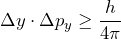$\Delta y \cdot \Delta p_y \geq \dfrac{h}{4\pi}$ holds (Kennard 1927, Robertson 1929). There is thus no preparation with simultaneously sharp position and momentum values. Importantly, this relation concerns the spreads, not the mean values. This is the version meant throughout this course.

Disturbance uncertainty: In a sequential measurement — position first, then momentum — one considers the disturbance that the position measurement causes in the momentum. This is exactly the picture underlying the Heisenberg microscope (Section 1): “You cannot measure the position without disturbing the momentum.” The same idea (“no measurement without disturbance”) is used, among other things, in quantum cryptography.

Measurement uncertainty: Sometimes a further distinction is drawn: measurement uncertainty. This concerns the joint, approximate measurement of two quantities — that is, position and momentum are to be measured simultaneously in a single measurement. Contrary to a common formulation of the uncertainty relation, this is in principle quite possible. For the resulting spreads in position and momentum, a relation of the same type holds again, but the joint measurement comes at the price of a factor of 2 in the product of the spreads of the measured values.

Crucial for teaching: The three statements are not identical. The Heisenberg microscope illustrates the disturbance variant, whereas the relation usually intended, $\Delta y \cdot \Delta p_y \geq \dfrac{h}{4\pi}$ , is the preparation variant. Historically, the two were often conflated. That a Heisenberg-type relation can be rigorously proven for measurement and disturbance uncertainty as well was only established more recently (Busch, Lahti & Werner, Phys. Rev. Lett. 111, 160405 (2013)).

2. Teaching the Uncertainty Relation

The didactic literature offers a number of approaches to teaching the uncertainty relation. These are briefly presented below, together with their respective advantages and disadvantages.

A more detailed discussion of the various approaches can be found in the article “Die Heisenberg´sche Unbestimmtheitsrelation im Unterricht” (Heisenberg’s uncertainty relation in the classroom) (published in “Physik in der Schule” 35 (1997), pp. 380–384).

1. The Heisenberg Microscope

Heisenberg himself used this thought experiment in the early years of quantum mechanics to illustrate his relation. It conveys the idea that the uncertainty relation has to do with a “disturbance” caused by a measurement. This measurement disturbance is indeed a real effect (disturbance uncertainty, see above); the relation usually intended, however, is the preparation uncertainty, which does not arise from a measurement at all. The microscope picture conflates the two — which is didactically problematic.

Core of the argument: If one attempts to determine the position of an electron by illuminating it with sufficiently short-wavelength light, the uncontrollable recoil of the scattered photon disturbs the electron’s momentum so much that the uncertainty relation is satisfied.

Disadvantage: This introduction almost inevitably leads students to imagine that, before the disturbance, the electron possessed both a definite position and a definite momentum. For if the measurement disturbs something (momentum), the electron must have possessed that something beforehand too. This line of argument thus leads back to classical notions.

2. Uncertainty of Wave Packets

Core of the statement: It is not possible to construct, by superposing waves from a limited range of wave numbers $\Delta k$ , wave packets whose spatial extent is smaller than $\dfrac{1}{\Delta k}$ . An uncertainty relation of the form $\Delta x \cdot \Delta k \approx 0,5$ thus holds. This is a fundamental theorem of Fourier theory, which can be demonstrated by superposing just a few partial waves.

Advantage: The demonstration is technically correct, since it makes no implicit use of classical-trajectory notions.

Disadvantage: It has nothing to do with quantum physics; it is a statement about the properties of the Fourier transform.

3. Potential Well

Core of the statement: The idea of working out the uncertainty relation for the one-dimensional, infinitely high potential well was suggested by Wegener.

Advantage: This approach works with the genuine quantum-mechanical standard deviation. It is not particularly involved and has the advantage that the correct quantum-mechanical concepts are used.

Disadvantage: Quantum-mechanical averaging must be introduced beforehand.

4. Diffraction at a Single Slit

Core of the statement: This thought experiment assumes that electrons with fixed momentum $p$ fall onto a screen with a slit of width $d$ . The characteristic diffraction pattern forms on the detection screen. The position uncertainty $\Delta x$ is equated with the slit width $d$ .

For the position of the first diffraction minima:

$\sin(\alpha) = \dfrac{\lambda}{\Delta x}$

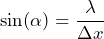
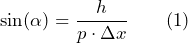
Substituting the de Broglie wavelength $\lambda = \dfrac{h}{p}$ associated with the electron beam into this equation gives:

$\sin(\alpha) = \dfrac{h}{p \cdot \Delta x} \qquad \text{(1)}$

The momentum uncertainty can be estimated from the angle $\alpha$ (the width of the central maximum), and:

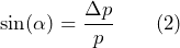
$\sin(\alpha) = \dfrac{\Delta p}{p} \qquad \text{(2)}$

From (1) and (2) one obtains the estimate $\Delta x \cdot \Delta p \gg h$ .

Disadvantage: The problem lies in inferring the spread of the momenta at the slit from the intensity distribution on the screen. The argument usually given easily leads to the notion that the electrons travel from the slit to the screen along a classical trajectory.

You can read about how to get from the momentum distribution at the slit to the position distribution on the screen in a quantum-mechanically correct way in the article “Zur Ableitung der Unbestimmtheitsrelation am Einzelspalt” (On deriving the uncertainty relation for a single slit).

5. Recommendation for Teaching

The statement that position and momentum cannot both be measured with arbitrary precision at the same time should be used with caution. The uncertainty relation does not, strictly speaking, concern simultaneous measurements. Here you will find classroom-appropriate information on precise and simultaneous measurements.

The interpretation of the Heisenberg uncertainty relation as a restriction on the possible ways of preparing certain pairs of properties is correct in any case. In terms of the property concept, one can state: quantum objects cannot be brought into a state in which they simultaneously have a definite position property and a definite momentum property.

For a quantitative derivation, the single-slit derivation and the potential-well method are good options.

Back