Optisches Quantencomputing
Überblicksvideo – Lernmaterial – Aufgaben – Weiterführende Informationen & Literatur – Quiz
Sollten dir Begriffe unklar sein, kannst du jederzeit im Glossar nachsehen.
Überblicksvideo
Lernmaterial
Die Wissenschaftler setzen große Erwartungen in das Quantencomputing. Es wird erwartet, dass Quantencomputer und darüber hinaus im Allgemeinen auch Quantentechnologien in der Lage sein werden, wichtige Probleme der heutigen Welt zu lösen, Moleküle zu modellieren und einige Arten von Berechnungen durchzuführen, zu denen klassische Computer niemals in der Lage sein werden oder zumindest nicht in einer angemessenen Zeit. Aber wie ist das möglich? Was ist der grundlegende Unterschied zwischen klassischem und Quantencomputing?
Einer der beiden grundlegenden Unterschiede ist die Quantenparallelität. Quantencomputer beruhen auf Qubits. Wie Bits im klassischen Rechnen enthalten Qubits die notwendigen Informationen, speichern sie und können ausgelesen werden, um auf die Informationen zuzugreifen. Im Gegensatz zu Bits können Qubits in Überlagerungszuständen von 0 und 1 existieren, und es können Interferenzen auftreten, die für bestimmte Aufgaben genutzt werden können. Weitere Informationen zur Interferenz sind in Grundprinzip 2 beschrieben:
Grundprinzip 2: Interferenz von einzelnen Quantenobjekten
Interferenz tritt auf, wenn es zwei oder mehr „Wege“ gibt, die zu demselben Versuchsergebnis führen. Keine der Alternativen ist dann im klassischen Sinn realisiert – die Quantenobjekte befinden sich in Überlagerungszuständen.
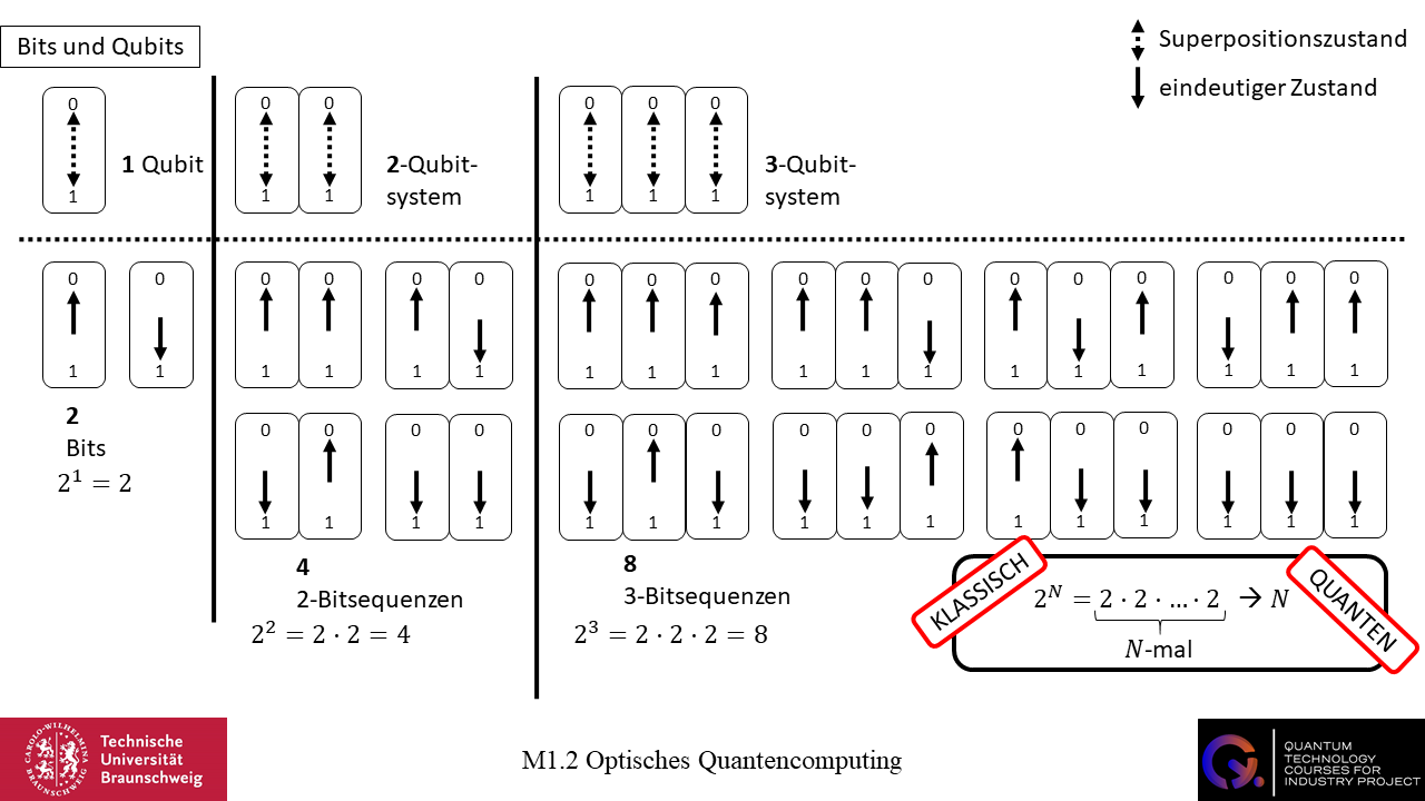
Für ein besseres Verständnis des Grundprinzips und der Quantenparallelität, diskutieren wir nun ein Beispiel. Hierzu vergleichen wir ein Bit – die Grundkomponente des klassischen Computings – mit einem Qubit – die Grundkomponente des Quantencomputings. Bei einer Messung kann es bei beiden Grundkomponenten, Bit und Qubit, zu zwei möglichen Zuständen bzw. Endergebnissen kommen: entweder 0 oder 1. Der Unterschied besteht darin, dass ein Qubit in einem Überlagerungszustand existieren kann. Bevor es gemessen wird, befindet sich ein Bit in einem diskreten Zustand. Es ist entweder 0 oder 1. Man führt eine Operation durch und misst das Bit. Das Ergebnis ist einer der beiden möglichen Zustände. Im Gegensatz dazu kann sich das Qubit in einem Überlagerungszustand befinden, d. h. es kann gleichzeitig in den beiden Zuständen 0 und 1 vorliegen. Man führt eine Operation durch, misst das Qubit und erhält einen der beiden möglichen Zustände. Wir brauchen also zwei klassische Bits, 0 und 1, um den Überlagerungszustand eines Qubits zu beschreiben. Aber wie viele klassische Bits brauchen wir, um weitere Multi-Qubit-Systeme zu beschreiben?
Werfen wir einen Blick auf ein 2-Bit-System. Es kann in vier möglichen Zuständen existieren; die 2-Bit-Sequenzen, die diese Zustände beschreiben, sind 00, 01, 10 und 11. Wir bräuchten also vier klassische 2-Bit-Sequenzen, um den Superpositionszustand eines 2-Qubit-Systems zu beschreiben. In einem Superpositionszustand kann ein 2-Qubit-System gleichzeitig in den Zuständen 00, 01, 10 und 11 existieren.
Werfen wir einen Blick auf ein 3-Bit-System. Es kann in acht möglichen Zuständen existieren; die 3-Bit-Sequenzen, die diese Zustände beschreiben, sind 000, 001, 010, 100, 011, 101, 110, 111. Wir benötigen also acht klassische 3-Bit-Sequenzen, um den Überlagerungszustand eines 3-Qubit-Systems zu beschreiben. In einem Superpositionszustand kann ein 3-Qubit-System gleichzeitig in den Zuständen 000, 001, 010, 100, 011, 101, 110, 111 existieren.
Wir wollen versuchen, eine allgemeine Aussage zu formulieren: Man kann sehen, dass sich die Anzahl der Bitfolgen verdoppelt, wenn man ein Qubit zum Multi-Qubit-System hinzufügt. Das liegt daran, dass sich die Zahl der möglichen Zustände verdoppelt, da die neuen Zustände aus allen vorherigen Zuständen mit einer zusätzlichen 0 und allen vorherigen Zuständen mit einer zusätzlichen 1 bestehen. Betrachten wir zum Beispiel den Übergang von einem Qubit zu einem 2-Qubit-System. Wir benötigen zwei klassische Bits, 0 und 1, um den Überlagerungszustand eines Qubits zu beschreiben. Wenn wir eine zusätzliche 0 zu diesen Zuständen hinzufügen, erhalten wir 00 und 01. Wenn wir eine zusätzliche 1 zu diesen Zuständen hinzufügen, erhalten wir 10 und 11. Insgesamt haben wir also vier 2-Bit-Sequenzen, 00, 01, 10, 11, die den Überlagerungszustand eines 2-Qubit-Systems beschreiben! In Analogie dazu beschreiben wir den Überlagerungszustand eines 3-Qubit-Systems, eines 4-Qubit-Systems und so weiter.
Schließlich benötigen wir  klassische Zustände, um den Überlagerungszustand eines N-Qubit-Systems zu beschreiben!
Dies ist die eingangs erwähnte Quantenparallelität. Sie hat zwar auf ein einzelnes Bit/Qubit so gut wie keine Auswirkung, unterscheidet aber bei einer Vielzahl von Bits/Qubits das Quantencomputing eindeutig vom klassischen Computing. Du solltest hierbei daran denken, dass wir von Überlagerungszuständen sprechen. Wie bereits im Grundprinzip 2 erwähnt, sind diese Zustände nicht im klassischen Sinne „realisiert“! Beim Messen besteht eine gewisse Wahrscheinlichkeit, einen der Zustände zu messen, die Teil des Überlagerungszustandes sind.
Dies erklärt aber noch nicht vollständig den Quantenvorteil. Auch wenn Qubits gleichzeitig in mehreren Zuständen existieren können, muss man letztlich immer noch einen Zustand messen. Der Quantenvorteil ergibt sich aus der Kontrolle von Interferenzprozessen, die es ermöglicht, die Ausgabe von Qubit-Systemen zu kontrollieren.
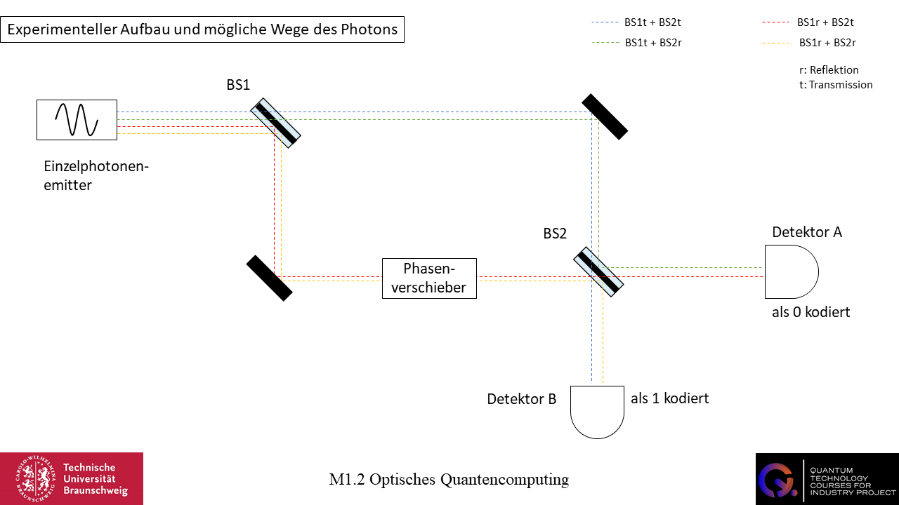
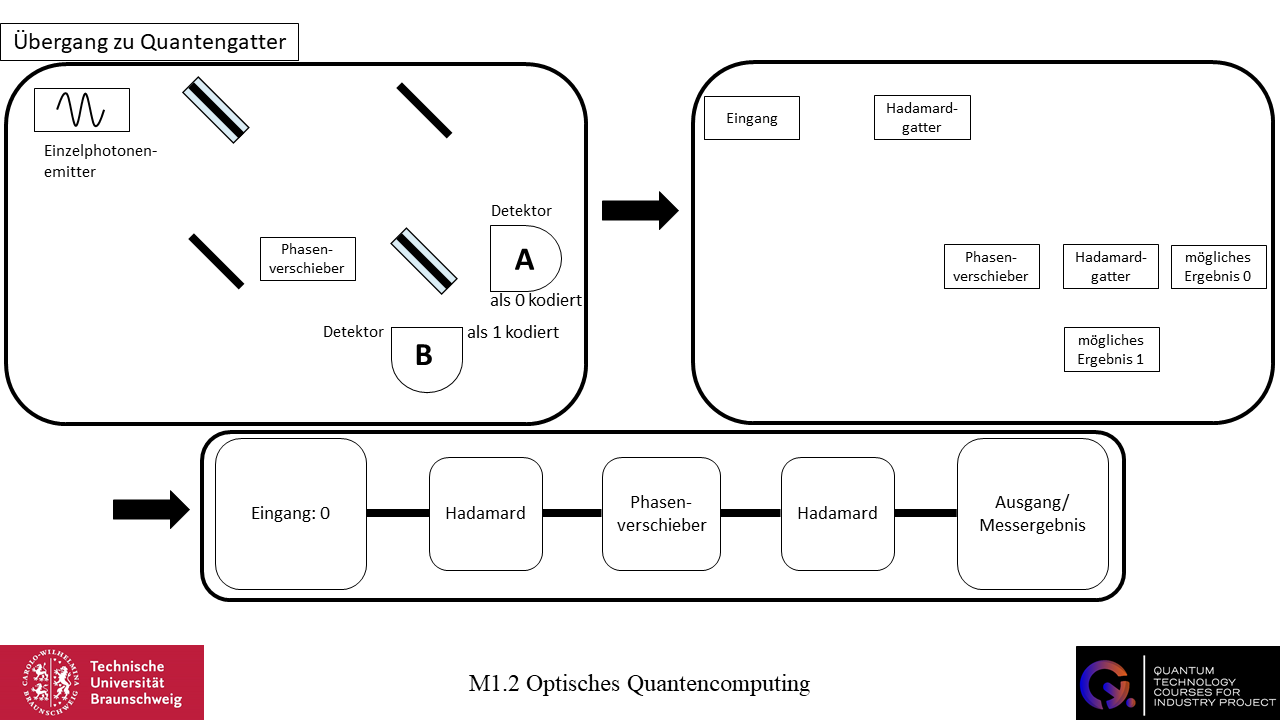
Aber was ist Interferenz? Vielleicht ist dir die Interferenz aus der Optik bekannt. Zwei Wellen (in der Optik dann zumeist Licht in Form von Laserstrahlen) können sich hier überlagern und erzeugen dann ein Muster. Lasst uns ein Experiment betrachten, dass dieses Phänomen erklärt. Für den Versuchsaufbau benötigen wir zwei Strahlenteiler, zwei Spiegel, zwei Detektoren, einen Einzelphotonenemitter und einen Phasenverschieber.
Die emittierten Einzelphotonen haben den Zustand  . Wenn Detektor A ein Photon detektiert, kodieren wir dies als , wenn Detektor B eines detektiert kodieren wir dies als
  . Vorerst hat unser Phasenverschieber nur zwei Zustände: entweder ist er deaktiviert und die Phasenverschiebung der ankommenden Wellen ist 0 (die Welle bleibt gleich), oder er ist aktiviert und die Phasenverschiebung der ankommenden Wellen ist
  (die Welle wird um die Hälfte ihrer Wellenlänge verschoben).
Mit diesem Versuchsaufbau sind wir nun in der Lage, Berechnungen durchzuführen und betreiben gewissermaßen optisches Quantencomputing. Zwischen dem Einzelphotonenemitter und den Detektoren kann das Photon als eine Welle beschrieben werden, die auch wellenhafte Eigenschaften hat. Das ist die Wellennatur von Quantenobjekten.
Um potenziell den Detektor A zu erreichen, hat das Photon zwei mögliche Wege. Auf beiden Wegen wird das Photon einmal transmittiert und einmal reflektiert! Unabhängig davon, welchen Weg das Photon „nimmt“, ist die Phasenverschiebung dieselbe.
Um möglicherweise den Detektor B zu erreichen, hat das Photon ebenfalls zwei mögliche Wege. Diesmal sind die Wege unterschiedlich. Auf dem ersten Weg wird das Photon zweimal transmittiert, auf dem zweiten Weg wird es einmal reflektiert und einmal transmittiert. Dadurch entsteht eine unveränderliche Phasenverschiebung, die für die weiteren Überlegungen wichtig sein wird.
Stellen wir die Pfade nach, die das Photon „durchläuft“. In Wirklichkeit können wir das nicht tun, weil sich das Photon in einem Überlagerungszustand befindet und wir bereits in Grundregel 2 erwähnt haben, dass in einem Überlagerungszustand die Alternativen nicht auf klassische Weise realisiert werden. Der Einfachheit halber wollen wir aber versuchen zu rekonstruieren, was das Photon „macht“.
Zunächst wird das Photon aus dem Emitter emittiert. Von hier aus „wandert“ es zum Strahlteiler. Am ersten Strahlteiler (BS1) gibt es zwei verschiedene Wege. Das Photon befindet sich nun in einer Überlagerung des Transmissionsweges und des Reflexionsweges. Wie in Grundprinzip 2 erwähnt, realisiert das Photon (Quantenobjekt) nicht beide Wege im klassischen Sinne. Eine Messung (durch Detektoren in beiden Pfaden) würde das Photon auf einem Pfad erfassen, nicht auf beiden Pfaden! Am zweiten Strahlteiler (BS2) gibt es wieder zwei verschiedene Pfade und das Photon existiert in einer Überlagerung von beiden. Letztendlich gibt es vier mögliche Pfade (BS1 t + BS2 t; BS1 r + BS2 t; BS1 t + BS2 r; BS1 r + BS2 r).
Betrachten wir die möglichen Wege zum Detektor A. Diese sind BS1 t + BS2 r und BS1 r + BS2 t, also zwei mögliche Wege. Bei den weiteren Überlegungen ist es wichtig zu bedenken, dass wir das Photon als Welle beschreiben können.
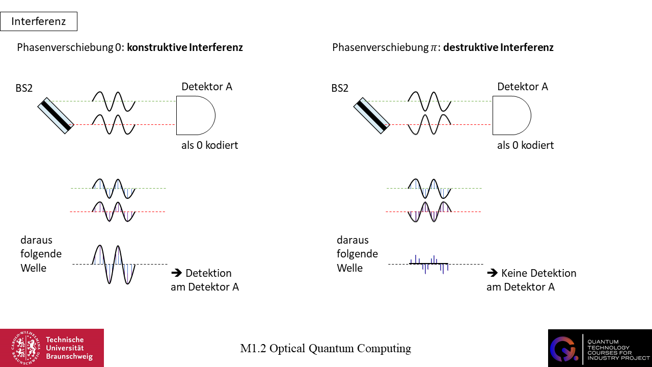
Unser Phasenverschieber ist deaktiviert, die Phasenverschiebung ist 0. Wenn wir nun einzelne Photonen aussenden (Zustand ), werden wir immer ein detektieren (d.h. Detektion am Detektor A). Dies ist auf die konstruktive Interferenz zurückzuführen. Auf dem Weg zwischen BS2 und Detektor A überschneiden sich die beiden möglichen Wege. Da wir das Photon als eine Welle beschreiben, bedeutet dies, dass sich zwei Wellen überlagern. Die Phasenverschiebung ist deaktiviert und die Pfade unterliegen den gleichen Bedingungen. Insgesamt haben beide Wellen die gleiche Phasenverschiebung, die Maxima und Minima beider Wellen überlagern sich und werden verstärkt. Die resultierende Welle hat größere Maxima und Minima und das Photon wird bei A erkannt.
Unser Phasenverschieber ist aktiviert, die Phasenverschiebung ist . Wenn wir nun einzelne Photonen aussenden (Zustand ), werden wir immer eine (d. h. Detektion am Detektor B) messen. Dies ist auf die destruktive Interferenz zurückzuführen. Auf dem Weg zwischen BS2 und Detektor A überschneiden sich die beiden möglichen Wege und somit ebenfalls die Wellen. Diesmal hat jedoch eine der Wellen aufgrund eines aktivierten Phasenverschiebers eine Phasenverschiebung von . Dies hat zur Folge, dass sich die Maxima der einen Welle mit den Minima der anderen Welle überlagern und umgekehrt. Die resultierende „Welle“ ist eine konstante Linie, ohne Maxima und Minima, und das Photon wird nicht bei A detektiert.
Ähnliche Schlussfolgerungen lassen sich für den Detektor B ziehen. Wenn der Phasenverschieber deaktiviert ist, detektiert Detektor B nichts. Wenn der Phasenverschieber aktiviert ist, detektiert Detektor B die Photonen.
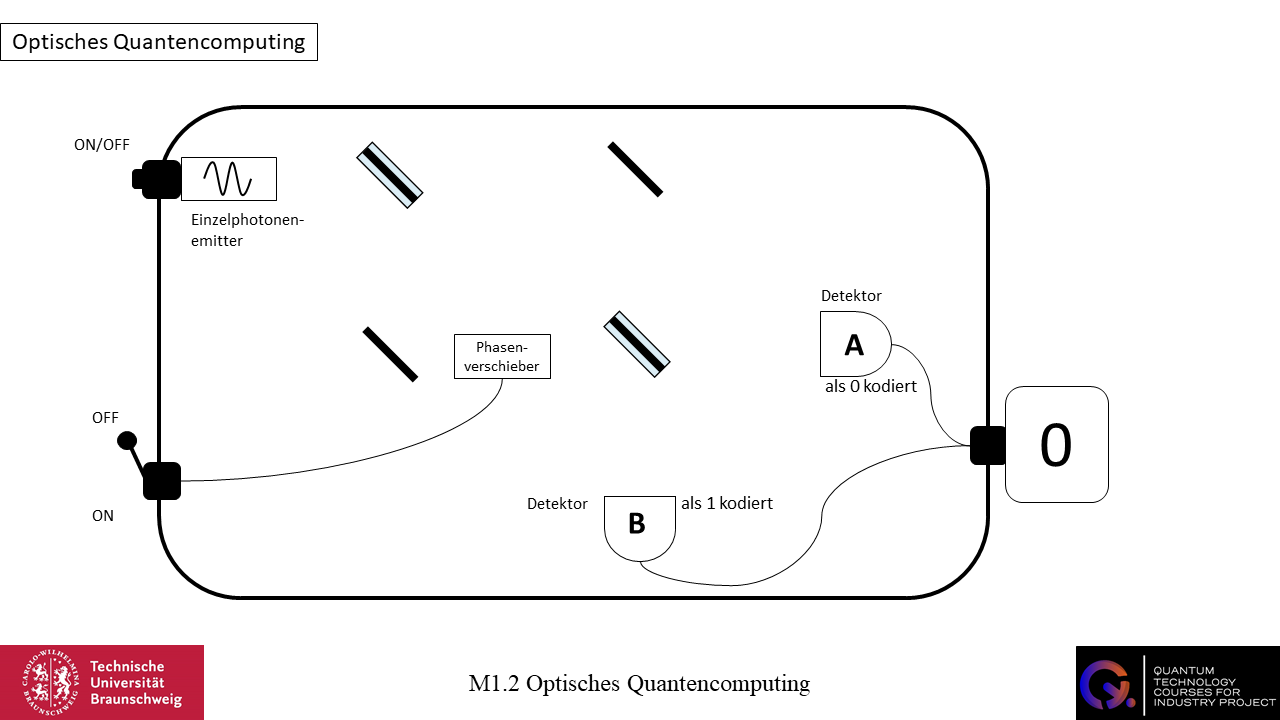
Der oben beschriebene Versuchsaufbau stellt das Mach-Zehnder-Interferometer dar. Im Hinblick auf das Quantencomputing könnte es potenziell für das optische Quantencomputing verwendet werden, mit einer ähnlichen Struktur wie in der Abbildung unten. Durch gezielte Steuerung der Phasenverschiebung der Pfade kann die Interferenz genutzt werden, um das Ergebnis einer Berechnung oder einer Qubit-Sequenz zu steuern.
Wie beim klassischen Rechnen verwenden wir Gatter, um die Struktur des Rechners zu beschreiben. Quantengatter sind schwierig zu realisieren. Wir werden nicht auf den mathematischen Hintergrund oder die technische Realisierung eingehen, da sie im Moment nicht wichtig sind und wir uns auf die qualitative Darstellung der Quantenphysik konzentrieren möchten.
Für unser vorheriges Beispiel benötigen wir ein Hadamardgatter und einen Phasenverschieber. Ein Hadamardgatter kann man sich wie einen Strahlteiler vorstellen. Es versetzt das Qubit in eine Überlagerung der Zustände und , so wie der Strahlteiler das Photon in eine Überlagerung der Pfade „oben“ und „unten“ versetzt.
Um das Mach-Zehnder-Interferometer im Sinne des Quantencomputers zu realisieren, benötigen wir zwei Hadamardgatter – analog zu zwei Strahlteilern – und den Phasenverschieber. Wenn wir den Phasenverschieber zwischen den beiden Hadamardgattern platzieren, haben wir genau die gleiche Situation wie im Mach-Zehnder-Interferometer. Durch die Steuerung des Phasenverschiebers können wir wiederum das Ergebnis kontrollieren.
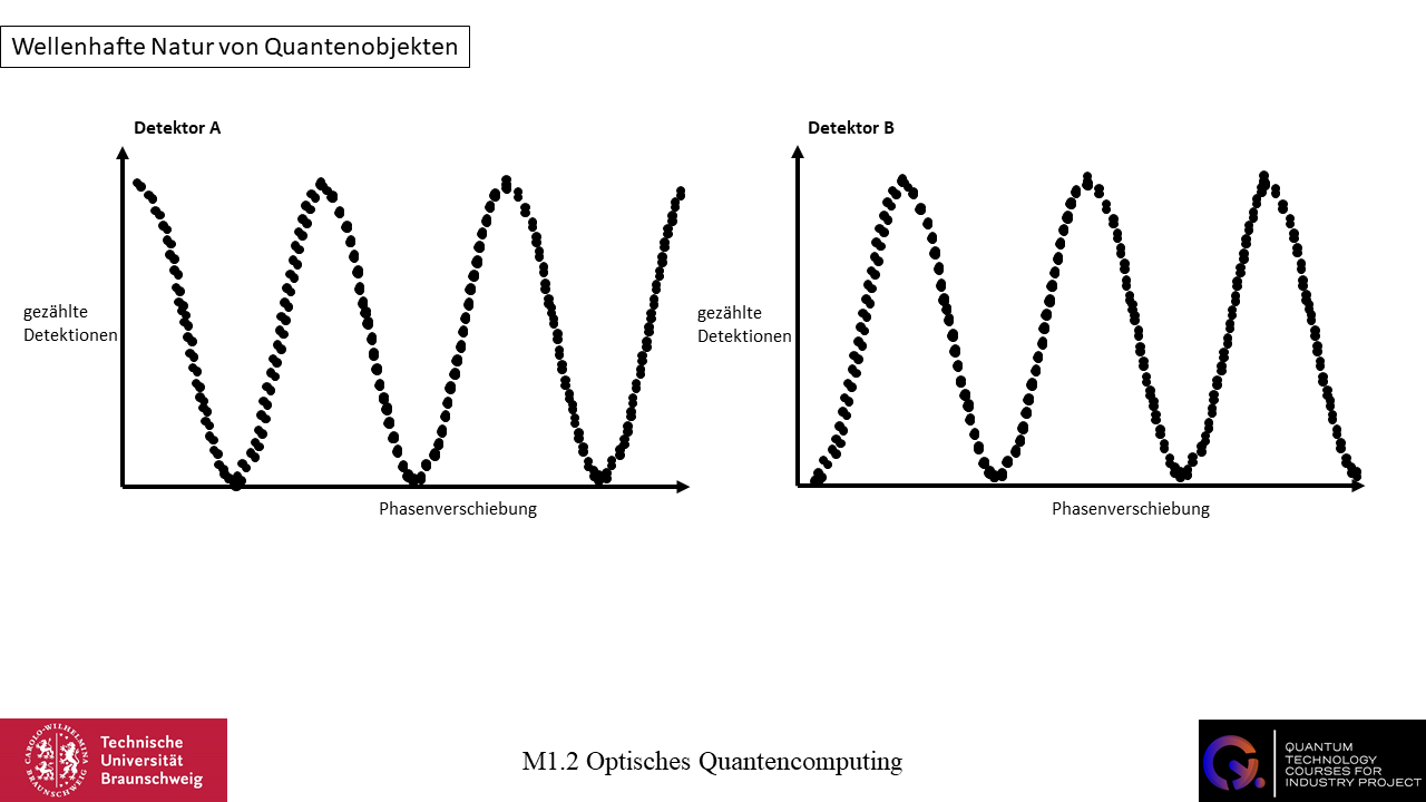
Interessanterweise lässt sich die wellenartige Natur von Quantenobjekten beobachten, wenn wir den Phasenverschieber auf flexiblere Weise variieren – und nicht nur zwischen zwei Zuständen der Phasenverschiebung unterscheiden. Die Abbildung zeigt dies. Hier sind die Zählungen als Funktion des Phasenschiebers aufgetragen, und wir sehen eine wellenförmige Funktion. Aber darauf gehen wir hier nicht ein, dies ist Teil des nächsten Themas!
Aufgaben
Aufgabe 1:
Benenne das Grundprinzip 2 und erkläre dessen Bedeutung.
Aufgabe 2:
Wiederhole das experimentelle Setup unseres optischen Quantencomputers und erkläre warum und wie es zur Interferenz kommt.
Aufgabe 3:
Nenne jede klassische 4-Bit-Sequenz in der ein 4-Qubit-System gleichzeitig existieren kann. Wie viele klassische Bit-Sequenzen werden benötigt um den Superpositionszustand eines 4-Qubit-Systems zu beschreiben?
Aufgabe 4:
Ein Supercomputer hat die Kapazität um in  Zuständen von Bit-Sequenzen zu existieren. Ermittle die Zahl N eines N-Qubit-Systems, welches in der gleichen Anzahl an Zuständen gleichzeitig existieren kann.
Lösungen:
Weiterführende Informationen & Literatur
Interferenz am Mach-Zehnder Interferometer: Grangier, P., Roger, G. & Aspect, A. (1986). Experimental Evidence for a Photon Anticorrelation Effect on a Beam Splitter: A New Light on Single-Photon Interferences. Europhysics Letters, 1(4), 173-179.
Mathematische Erklärung der Einzelqubitinterferenz: Youtube-Video & https://qubit.guide/2.4-single-qubit-interference.html
Quantengravimeter, ein Video von Atomionics: Youtube-Video
Quantengravimeter, ein Artikel: Menoret, V., Le Moigne, N., Bonvalot, S., Bouyer, P., Landragin, A. & Desruelle, B. (2018). Gravity measurements below 10^-9 g with a transportable absolute quantum gravimeter. Scientific Reports, 8:12300. DOI: 10.1038/s41598-018-30608-1.
Müller, R. & Greinert, F. (2023). Quantentechnologien: Für Ingenieure. De Gruyter.
Qiang, X., Zhou, X., Wang, J., Wilkes, C.M., Loke, T., O’Gara, S., Kling, L., Marshall, G.D., Santagati, R., Ralph, T.C., Wang, J.B., O’Brien, J.L., Thompson, M.G. & Matthews, J.C.F. (2018). Large-scale silicon quantum photonics implementing arbitrary two-qubit processing. Nature Photo, 12. 534-539. doi: https://doi.org/10.1038/s41566-018-0236-y
(No author) (n.Y.). 2.4 Single qubit interference: Introduction. Online: https://qubit.guide/2.4-single-qubit-interference.html. [last access: 07-08-2023].