Three-dimensional infinite potential well

1. One-dimensional potential well

The infinitely high potential well is one of the simplest quantum-mechanical systems. The wave functions for the potential well are usually obtained from the analogy with a standing wave. The wave function is required to vanish at the edges of the potential well (at $x = 0$ and $x = a$ ). Then only very specific de Broglie wavelengths “fit” into this region. “Standing electron waves” form, such that exactly an integer multiple of half the de Broglie wavelength fits into the distance $a$ :

$\lambda_n = \dfrac{2a}{n} \qquad (n = 1,2,3,...)$

This means that not every de Broglie wavelength is allowed inside the potential well. The wave function belonging to the $n$ -th state is:

$\psi_n = \sin\biggl(\dfrac{2\pi}{\lambda_n}x\biggr) = \sin\biggl(\dfrac{n\pi}{a}x\biggr)$

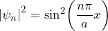
The corresponding probability density (the squared modulus of the wave function) is:

$\left| \psi_n \right|^2 = \sin^2\biggl(\dfrac{n\pi}{a}x\biggr)$

Determining the energy:

The energy levels are usually determined from the allowed wavelengths using the de Broglie relation $\lambda = \dfrac{h}{p}$ :

$\begin{array}{ll} W &= W_{kin} + W_{pot} = W_{kin} + 0 \\[2ex] &= \dfrac{p^2}{2m} = \dfrac{h^2}{2m\lambda^2} \end{array}$

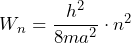
Substituting the formula for $\lambda_n$ obtained above gives the energy levels of an electron in the potential well:

$W_n = \dfrac{h^2}{8ma^2} \cdot n^2$

2. Three-dimensional potential well

Having dealt with the one-dimensional potential well, the three-dimensional potential well no longer poses a problem, since the reasoning above can simply be repeated separately for each of the three spatial dimensions. The wave function is the product of three sine functions, one for each spatial direction:

$\psi_{n_x n_y n_z} (x,y,z) = \sin\biggl(\dfrac{n_x \pi}{a} x \biggr) \sin\biggl(\dfrac{n_y \pi}{a} y \biggr) \sin\biggl(\dfrac{n_z \pi}{a} z \biggr)$

The energy is composed accordingly:

$W = \dfrac{p^2_x + p^2_y + p^2_z}{2m} = \dfrac{h^2}{8ma^2} (n^2_x + n^2_y + n^2_z)$

This is the result needed in the main text.

3. Treatment using the Schrödinger equation

Once the Schrödinger equation (cf. Chapter 8.8) has been made plausible and introduced in class, its solution for the case of the potential well is very simple. Inside the potential well, this is simply the equation for a free particle:

$- \dfrac{\hbar^2}{2m} \dfrac{d^2}{dx^2} \psi (x) = E \psi (x)$

Substituting the ansatz

$\psi (x) = A \cdot \sin(kx)$
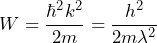
into this equation gives:

$W = \dfrac{\hbar^2 k^2}{2m} = \dfrac{h^2}{2m\lambda^2}$

The boundary conditions (the wave function vanishing at $x = 0$ and $x = a$ ) lead to the same condition as above:

$\lambda_n = \dfrac{2a}{n}$
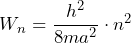
This again gives the energy levels in the potential well as above:
$W_n = \dfrac{h^2}{8ma^2}\cdot n^2$

Back to the chapter overview.